# Import the following libraries
# For fetching from the Raster API
import requests
# For making maps
import folium
import folium.plugins
from folium import Map, TileLayer
# For talking to the STAC API
from pystac_client import Client
# For working with data
import pandas as pd
# For making time series
import matplotlib.pyplot as plt
# For formatting date/time data
import datetime
# Custom functions for working with GHGC data via the API
import ghgc_utilsGOSAT-based Top-down Total and Natural Methane Emissions
Total and wetland yearly methane emissions derived using the GEOS-Chem global chemistry transport model with inclusion of GOSAT data for 2010 to 2022 on a 4°(latitude) x 5°(longitude) grid
Access this Notebook
You can launch this notebook in the US GHG Center JupyterHub (requires access) by clicking the following link: GOSAT-based Top-down Total and Natural Methane Emissions. If you are a new user, you should first sign up for the hub by filling out this request form and providing the required information.
If you do not have a US GHG Center Jupyterhub account, you can access this notebook through MyBinder by clicking the button below.
![]()
Table of Contents
Data Summary and Application
- Spatial coverage: Global
- Spatial resolution: 4° x 5°
- Temporal extent: 2010 - 2022
- Temporal resolution: Annual
- Unit: Teragrams of methane per year (Tg CH₄/year)
- Utility: Climate Research
For more information, visit the GOSAT-based Top-down Total and Natural Methane Emissions data overview page.
Approach
- Identify available dates and temporal frequency of observations for the given collection using the US Greenhouse Gas Center (GHGC) Application Programming Interface (API)
/stacendpoint. The collection processed in this notebook is the GOSAT-based Top-down Total and Natural Methane Emissions data product. - Pass the STAC item into the raster API /collections/{collection_id}/items/{item_id}/{tile_matrix_set_id}/tilejson.json endpoint.
- Using
folium.plugins.DualMap, visualize two tiles (side-by-side), allowing time point comparison. - After the visualization, perform zonal statistics for a given polygon.
About the Data
GOSAT-based Top-down Total and Natural Methane Emissions
The NASA Carbon Monitoring System Flux (CMS-Flux) team analyzed remote sensing observations from Japan’s Greenhouse gases Observing SATellite (GOSAT) to produce the global Committee on Earth Observation Satellites (CEOS) CH₄ Emissions data product. They used an analytic Bayesian inversion approach and the GEOS-Chem global chemistry transport model to quantify annual methane (CH₄) emissions and their uncertainties at a spatial resolution of 1° by 1° and then projected these to each country for 2019.
For more information regarding this dataset, please visit the GOSAT-based Top-down Total and Natural Methane Emissions data overview page.
Terminology
Navigating data via the US Greenhouse Gas Center (GHGC) Application Programming Interface (API), you will encounter terminology that is different from browsing in a typical filesystem. We’ll define some terms here which are used throughout this notebook.
catalog: All datasets available at the/stacendpointcollection: A specific dataset, e.g. GOSAT-based Top-down Total and Natural Methane Emissionsitem: One data file (i.e. granule) in the dataset, e.g. one annual file of fluxesasset: A variable available within the granule, e.g. anthropogenic methane emissionsSTAC API: SpatioTemporal Asset Catalogs - Endpoint for fetching metadata about available datasetsRaster API: Endpoint for fetching data itself, for imagery and statistics
Install the Required Libraries
The libraries below allow better execution of a query in the US GHG Center Spatio Temporal Asset Catalog (STAC) Application Programming Interface (API), where the granules for this collection are stored. You will learn the functionality of each library throughout the notebook.
Required libraries are pre-installed on the US GHG Center Hub. If you need to run this notebook elsewhere, please install them with this line in a code cell:
%pip install requests folium rasterstats pystac_client pandas matplotlib –quiet
Query the STAC API
STAC API Collection Names
Now, you must fetch the dataset from the US GHG Center STAC API by defining its associated STAC API collection ID as a variable. The collection ID, also known as the collection name, for the GOSAT-based Total and Wetland CH₄ Emissions dataset is gosat-based-ch4budget-yeargrid-v1.
# Provide STAC and RASTER API endpoints
STAC_API_URL = "https://earth.gov/ghgcenter/api/stac"
RASTER_API_URL = "https://earth.gov/ghgcenter/api/raster"

# Please use the collection name similar to the one used in STAC collection.

# Name of the collection for gosat budget methane.
collection_name = "gosat-based-ch4budget-yeargrid-v1"
# Using PySTAC client
# Fetch the collection from the STAC API using the appropriate endpoint
# The 'pystac' library makes an HTTP request
catalog = Client.open(STAC_API_URL)
collection = catalog.get_collection(collection_name)
# Print the properties of the collection to the console
collection- type "Collection"
- id "gosat-based-ch4budget-yeargrid-v1"
- stac_version "1.1.0"
- description "As part of the global stock take (GST), countries are asked to provide a record of their greenhouse gas (GHG) emissions to inform decisions on how to reduce GHG emissions. The NASA Carbon Monitoring System Flux (CMS-Flux) team has used remote sensing observations from Japan's Greenhouse gases Observing SATellite (GOSAT) to produce modeled total methane (CH₄) emissions and uncertainties on a 1 degree by 1 degree resolution grid for the year 2019. The GOSAT data is used in the model to inform total emission estimates, as well as wetland (the primary natural source of methane), and various human-related sources such as fossil fuel extraction, transport, agriculture, waste, and fires. A prior GHG emission estimate (and assocated uncertainty) is provided for each layer, which is the emissions estimate without GOSAT data. The posterior GHG emission layers are informed by GOSAT total column methane data. An advanced mathematical approach is used with a global chemistry transport model to quantify annual CH₄ emissions and uncertainties. These estimates are expressed in teragrams of CH₄ per year (Tg/yr). The source data can be found at https://doi.org/10.5281/zenodo.8306874 and more information can also be found on the CEOS website https://ceos.org/gst/methane.html"
links[] 5 items
0
- rel "items"
- href "https://earth.gov/ghgcenter/api/stac/collections/gosat-based-ch4budget-yeargrid-v1/items"
- type "application/geo+json"
1
- rel "parent"
- href "https://earth.gov/ghgcenter/api/stac/"
- type "application/json"
2
- rel "root"
- href "https://earth.gov/ghgcenter/api/stac"
- type "application/json"
- title "US GHG Center STAC API"
3
- rel "self"
- href "https://earth.gov/ghgcenter/api/stac/collections/gosat-based-ch4budget-yeargrid-v1"
- type "application/json"
4
- rel "http://www.opengis.net/def/rel/ogc/1.0/queryables"
- href "https://earth.gov/ghgcenter/api/stac/collections/gosat-based-ch4budget-yeargrid-v1/queryables"
- type "application/schema+json"
- title "Queryables"
stac_extensions[] 2 items
- 0 "https://stac-extensions.github.io/render/v1.0.0/schema.json"
- 1 "https://stac-extensions.github.io/item-assets/v1.0.0/schema.json"
renders
dashboard
assets[] 1 items
- 0 "post-total"
rescale[] 1 items
0[] 2 items
- 0 0
- 1 3
- colormap_name "spectral_r"
post-anth
assets[] 1 items
- 0 "post-anth"
rescale[] 1 items
0[] 2 items
- 0 0
- 1 1
- colormap_name "spectral_r"
post-total
assets[] 1 items
- 0 "post-total"
rescale[] 1 items
0[] 2 items
- 0 0
- 1 3
- colormap_name "spectral_r"
prior-anth
assets[] 1 items
- 0 "prior-anth"
rescale[] 1 items
0[] 2 items
- 0 0
- 1 1
- colormap_name "spectral_r"
post-wetland
assets[] 1 items
- 0 "post-wetland"
rescale[] 1 items
0[] 2 items
- 0 0
- 1 1
- colormap_name "spectral_r"
prior-wetland
assets[] 1 items
- 0 "prior-wetland"
rescale[] 1 items
0[] 2 items
- 0 0
- 1 1
- colormap_name "spectral_r"
item_assets
post-anth
- type "image/tiff; application=geotiff; profile=cloud-optimized"
roles[] 2 items
- 0 "data"
- 1 "layer"
- title "Anthropogenic Posterior Methane Emissions"
- description "Methane emissions per grid cell from anthropogenic estimated by various inventories or models, excluding satellite based observations from GOSAT."
post-total
- type "image/tiff; application=geotiff; profile=cloud-optimized"
roles[] 2 items
- 0 "data"
- 1 "layer"
- title "Posterior Total Methane Emissions"
- description "Estimated total methane emissions per grid cell informed by GOSAT satellite total column methane data."
prior-anth
- type "image/tiff; application=geotiff; profile=cloud-optimized"
roles[] 2 items
- 0 "data"
- 1 "layer"
- title "Anthropogenic Prior Methane emissions"
- description "Methane emissions per grid cell from anthropogenic estimated by various inventories or models, excluding satellite based observations from GOSAT."
post-wetland
- type "image/tiff; application=geotiff; profile=cloud-optimized"
roles[] 2 items
- 0 "data"
- 1 "layer"
- title "Wetland Posterior Methane Emissions"
- description "Estimated methane emissions per grid cell from wetlands informed by GOSAT satellite total column methane data."
prior-wetland
- type "image/tiff; application=geotiff; profile=cloud-optimized"
roles[] 2 items
- 0 "data"
- 1 "layer"
- title "Wetland Prior Methane Emissions"
- description "Methane emissions per grid cell from wetlands estimated by various inventories or models, excluding satellite based observations from GOSAT."
- dashboard:is_periodic False
- dashboard:time_density "year"
- title "GOSAT-based Top-down Total and Natural Methane Emissions v1"
extent
spatial
bbox[] 1 items
0[] 4 items
- 0 -182.5
- 1 -90.9777777777778
- 2 177.5
- 3 90.97777777777777
temporal
interval[] 1 items
0[] 2 items
- 0 "2010-01-01T00:00:00Z"
- 1 "2022-01-01T00:00:00Z"
- license "CC-BY-4.0"
summaries
datetime[] 13 items
- 0 "2010-01-01T00:00:00Z"
- 1 "2011-01-01T00:00:00Z"
- 2 "2012-01-01T00:00:00Z"
- 3 "2013-01-01T00:00:00Z"
- 4 "2014-01-01T00:00:00Z"
- 5 "2015-01-01T00:00:00Z"
- 6 "2016-01-01T00:00:00Z"
- 7 "2017-01-01T00:00:00Z"
- 8 "2018-01-01T00:00:00Z"
- 9 "2019-01-01T00:00:00Z"
- 10 "2020-01-01T00:00:00Z"
- 11 "2021-01-01T00:00:00Z"
- 12 "2022-01-01T00:00:00Z"
Examining the contents of our collection under the temporal variable, we see that the data is available from January 2010 to December 2022. By looking at the dashboard:time density, we observe that the data is annual over that time period.
items = list(collection.get_items())  # Convert the iterator to a list
print(f"Found {len(items)} items")
Found 13 items# Examine the first item in the collection
items[0]- type "Feature"
- stac_version "1.1.0"
stac_extensions[] 2 items
- 0 "https://stac-extensions.github.io/raster/v1.1.0/schema.json"
- 1 "https://stac-extensions.github.io/projection/v2.0.0/schema.json"
- id "gosat-based-ch4budget-yeargrid-v1-2022"
geometry
- type "Polygon"
coordinates[] 1 items
0[] 5 items
0[] 2 items
- 0 -182.5
- 1 -90.9777777777778
1[] 2 items
- 0 177.5
- 1 -90.9777777777778
2[] 2 items
- 0 177.5
- 1 90.97777777777777
3[] 2 items
- 0 -182.5
- 1 90.97777777777777
4[] 2 items
- 0 -182.5
- 1 -90.9777777777778
bbox[] 4 items
- 0 -182.5
- 1 -90.9777777777778
- 2 177.5
- 3 90.97777777777777
properties
- datetime "2022-01-01T00:00:00Z"
links[] 5 items
0
- rel "collection"
- href "https://earth.gov/ghgcenter/api/stac/collections/gosat-based-ch4budget-yeargrid-v1"
- type "application/json"
1
- rel "parent"
- href "https://earth.gov/ghgcenter/api/stac/collections/gosat-based-ch4budget-yeargrid-v1"
- type "application/json"
2
- rel "root"
- href "https://earth.gov/ghgcenter/api/stac"
- type "application/json"
- title "US GHG Center STAC API"
3
- rel "self"
- href "https://earth.gov/ghgcenter/api/stac/collections/gosat-based-ch4budget-yeargrid-v1/items/gosat-based-ch4budget-yeargrid-v1-2022"
- type "application/geo+json"
4
- rel "preview"
- href "https://earth.gov/ghgcenter/api/raster/collections/gosat-based-ch4budget-yeargrid-v1/items/gosat-based-ch4budget-yeargrid-v1-2022/WebMercatorQuad/map?assets=post-total&rescale=0%2C3&colormap_name=spectral_r"
- type "text/html"
- title "Map of Item"
assets
post-anth
- href "s3://ghgc-data-store/gosat-based-ch4budget-yeargrid-v1/Post_Total_ANTH_CH4_emissions_2022.tif"
- type "image/tiff; application=geotiff"
- title "Anthropogenic Posterior Methane Emissions"
- description "Estimated methane emissions per grid cell from anthropogenic informed by GOSAT satellite total column methane data."
proj:bbox[] 4 items
- 0 -182.5
- 1 -90.9777777777778
- 2 177.5
- 3 90.97777777777777
- proj:wkt2 "GEOGCS["WGS 84",DATUM["WGS_1984",SPHEROID["WGS 84",6378137,298.257223563,AUTHORITY["EPSG","7030"]],AUTHORITY["EPSG","6326"]],PRIMEM["Greenwich",0,AUTHORITY["EPSG","8901"]],UNIT["degree",0.0174532925199433,AUTHORITY["EPSG","9122"]],AXIS["Latitude",NORTH],AXIS["Longitude",EAST],AUTHORITY["EPSG","4326"]]"
proj:shape[] 2 items
- 0 46
- 1 72
raster:bands[] 1 items
0
- scale 1.0
- nodata -9999.0
- offset 0.0
- sampling "area"
- data_type "float64"
histogram
- max 7.221596690004756
- min -4.446999177355341
- count 11
buckets[] 10 items
- 0 1
- 1 1
- 2 3
- 3 2954
- 4 284
- 5 41
- 6 15
- 7 6
- 8 5
- 9 2
statistics
- mean 0.11414124629900693
- stddev 0.4784569130920799
- maximum 7.221596690004756
- minimum -4.446999177355341
- valid_percent 100.0
proj:geometry
- type "Polygon"
coordinates[] 1 items
0[] 5 items
0[] 2 items
- 0 -182.5
- 1 -90.9777777777778
1[] 2 items
- 0 177.5
- 1 -90.9777777777778
2[] 2 items
- 0 177.5
- 1 90.97777777777777
3[] 2 items
- 0 -182.5
- 1 90.97777777777777
4[] 2 items
- 0 -182.5
- 1 -90.9777777777778
proj:transform[] 9 items
- 0 5.0
- 1 0.0
- 2 -182.5
- 3 0.0
- 4 -3.9555555555555557
- 5 90.97777777777777
- 6 0.0
- 7 0.0
- 8 1.0
roles[] 2 items
- 0 "data"
- 1 "layer"
post-total
- href "s3://ghgc-data-store/gosat-based-ch4budget-yeargrid-v1/Post_Total_TOTAL_CH4_emissions_2022.tif"
- type "image/tiff; application=geotiff"
- title "Posterior Total Methane Emissions"
- description "Estimated total methane emissions per grid cell informed by GOSAT satellite total column methane data."
proj:bbox[] 4 items
- 0 -182.5
- 1 -90.9777777777778
- 2 177.5
- 3 90.97777777777777
- proj:wkt2 "GEOGCS["WGS 84",DATUM["WGS_1984",SPHEROID["WGS 84",6378137,298.257223563,AUTHORITY["EPSG","7030"]],AUTHORITY["EPSG","6326"]],PRIMEM["Greenwich",0,AUTHORITY["EPSG","8901"]],UNIT["degree",0.0174532925199433,AUTHORITY["EPSG","9122"]],AXIS["Latitude",NORTH],AXIS["Longitude",EAST],AUTHORITY["EPSG","4326"]]"
proj:shape[] 2 items
- 0 46
- 1 72
raster:bands[] 1 items
0
- scale 1.0
- nodata -9999.0
- offset 0.0
- sampling "area"
- data_type "float64"
histogram
- max 8.355603568623742
- min -4.4208666115704
- count 11
buckets[] 10 items
- 0 1
- 1 1
- 2 2
- 3 3064
- 4 176
- 5 36
- 6 15
- 7 11
- 8 4
- 9 2
statistics
- mean 0.17184094844139713
- stddev 0.609173348963156
- maximum 8.355603568623742
- minimum -4.4208666115704
- valid_percent 100.0
proj:geometry
- type "Polygon"
coordinates[] 1 items
0[] 5 items
0[] 2 items
- 0 -182.5
- 1 -90.9777777777778
1[] 2 items
- 0 177.5
- 1 -90.9777777777778
2[] 2 items
- 0 177.5
- 1 90.97777777777777
3[] 2 items
- 0 -182.5
- 1 90.97777777777777
4[] 2 items
- 0 -182.5
- 1 -90.9777777777778
proj:transform[] 9 items
- 0 5.0
- 1 0.0
- 2 -182.5
- 3 0.0
- 4 -3.9555555555555557
- 5 90.97777777777777
- 6 0.0
- 7 0.0
- 8 1.0
roles[] 2 items
- 0 "data"
- 1 "layer"
prior-anth
- href "s3://ghgc-data-store/gosat-based-ch4budget-yeargrid-v1/Post_Total_ANTHP_CH4_emissions_2022.tif"
- type "image/tiff; application=geotiff"
- title "Anthropogenic Prior Methane Emissions"
- description "Estimated methane emissions per grid cell from anthropogenic informed by GOSAT satellite total column methane data."
proj:bbox[] 4 items
- 0 -182.5
- 1 -90.9777777777778
- 2 177.5
- 3 90.97777777777777
- proj:wkt2 "GEOGCS["WGS 84",DATUM["WGS_1984",SPHEROID["WGS 84",6378137,298.257223563,AUTHORITY["EPSG","7030"]],AUTHORITY["EPSG","6326"]],PRIMEM["Greenwich",0,AUTHORITY["EPSG","8901"]],UNIT["degree",0.0174532925199433,AUTHORITY["EPSG","9122"]],AXIS["Latitude",NORTH],AXIS["Longitude",EAST],AUTHORITY["EPSG","4326"]]"
proj:shape[] 2 items
- 0 46
- 1 72
raster:bands[] 1 items
0
- scale 1.0
- nodata -9999.0
- offset 0.0
- sampling "area"
- data_type "float64"
histogram
- max 6.610429486472943
- min 0.0
- count 11
buckets[] 10 items
- 0 3158
- 1 95
- 2 31
- 3 13
- 4 3
- 5 4
- 6 5
- 7 1
- 8 0
- 9 2
statistics
- mean 0.10766109705438384
- stddev 0.39201492749800015
- maximum 6.610429486472943
- minimum 0.0
- valid_percent 100.0
proj:geometry
- type "Polygon"
coordinates[] 1 items
0[] 5 items
0[] 2 items
- 0 -182.5
- 1 -90.9777777777778
1[] 2 items
- 0 177.5
- 1 -90.9777777777778
2[] 2 items
- 0 177.5
- 1 90.97777777777777
3[] 2 items
- 0 -182.5
- 1 90.97777777777777
4[] 2 items
- 0 -182.5
- 1 -90.9777777777778
proj:transform[] 9 items
- 0 5.0
- 1 0.0
- 2 -182.5
- 3 0.0
- 4 -3.9555555555555557
- 5 90.97777777777777
- 6 0.0
- 7 0.0
- 8 1.0
roles[] 2 items
- 0 "data"
- 1 "layer"
post-wetland
- href "s3://ghgc-data-store/gosat-based-ch4budget-yeargrid-v1/Post_Total_WET_CH4_emissions_2022.tif"
- type "image/tiff; application=geotiff"
- title "Wetland Posterior Methane Emissions"
- description "Estimated methane emissions per grid cell from wetlands informed by GOSAT satellite total column methane data."
proj:bbox[] 4 items
- 0 -182.5
- 1 -90.9777777777778
- 2 177.5
- 3 90.97777777777777
- proj:wkt2 "GEOGCS["WGS 84",DATUM["WGS_1984",SPHEROID["WGS 84",6378137,298.257223563,AUTHORITY["EPSG","7030"]],AUTHORITY["EPSG","6326"]],PRIMEM["Greenwich",0,AUTHORITY["EPSG","8901"]],UNIT["degree",0.0174532925199433,AUTHORITY["EPSG","9122"]],AXIS["Latitude",NORTH],AXIS["Longitude",EAST],AUTHORITY["EPSG","4326"]]"
proj:shape[] 2 items
- 0 46
- 1 72
raster:bands[] 1 items
0
- scale 1.0
- nodata -9999.0
- offset 0.0
- sampling "area"
- data_type "float64"
histogram
- max 8.256931476495279
- min -0.0016259006808810538
- count 11
buckets[] 10 items
- 0 3263
- 1 30
- 2 8
- 3 4
- 4 4
- 5 1
- 6 0
- 7 1
- 8 0
- 9 1
statistics
- mean 0.057699702142390175
- stddev 0.30538996981278377
- maximum 8.256931476495279
- minimum -0.0016259006808810538
- valid_percent 100.0
proj:geometry
- type "Polygon"
coordinates[] 1 items
0[] 5 items
0[] 2 items
- 0 -182.5
- 1 -90.9777777777778
1[] 2 items
- 0 177.5
- 1 -90.9777777777778
2[] 2 items
- 0 177.5
- 1 90.97777777777777
3[] 2 items
- 0 -182.5
- 1 90.97777777777777
4[] 2 items
- 0 -182.5
- 1 -90.9777777777778
proj:transform[] 9 items
- 0 5.0
- 1 0.0
- 2 -182.5
- 3 0.0
- 4 -3.9555555555555557
- 5 90.97777777777777
- 6 0.0
- 7 0.0
- 8 1.0
roles[] 2 items
- 0 "data"
- 1 "layer"
prior-wetland
- href "s3://ghgc-data-store/gosat-based-ch4budget-yeargrid-v1/Post_Total_WETP_CH4_emissions_2022.tif"
- type "image/tiff; application=geotiff"
- title "Wetland Prior Methane Emissions"
- description "Methane emissions per grid cell from wetlands estimated by various inventories or models, excluding satellite based observations from GOSAT."
proj:bbox[] 4 items
- 0 -182.5
- 1 -90.9777777777778
- 2 177.5
- 3 90.97777777777777
- proj:wkt2 "GEOGCS["WGS 84",DATUM["WGS_1984",SPHEROID["WGS 84",6378137,298.257223563,AUTHORITY["EPSG","7030"]],AUTHORITY["EPSG","6326"]],PRIMEM["Greenwich",0,AUTHORITY["EPSG","8901"]],UNIT["degree",0.0174532925199433,AUTHORITY["EPSG","9122"]],AXIS["Latitude",NORTH],AXIS["Longitude",EAST],AUTHORITY["EPSG","4326"]]"
proj:shape[] 2 items
- 0 46
- 1 72
raster:bands[] 1 items
0
- scale 1.0
- nodata -9999.0
- offset 0.0
- sampling "area"
- data_type "float64"
histogram
- max 6.639171063899994
- min 0.0
- count 11
buckets[] 10 items
- 0 3270
- 1 24
- 2 7
- 3 4
- 4 2
- 5 1
- 6 2
- 7 1
- 8 0
- 9 1
statistics
- mean 0.044958096379183715
- stddev 0.25345413829587626
- maximum 6.639171063899994
- minimum 0.0
- valid_percent 100.0
proj:geometry
- type "Polygon"
coordinates[] 1 items
0[] 5 items
0[] 2 items
- 0 -182.5
- 1 -90.9777777777778
1[] 2 items
- 0 177.5
- 1 -90.9777777777778
2[] 2 items
- 0 177.5
- 1 90.97777777777777
3[] 2 items
- 0 -182.5
- 1 90.97777777777777
4[] 2 items
- 0 -182.5
- 1 -90.9777777777778
proj:transform[] 9 items
- 0 5.0
- 1 0.0
- 2 -182.5
- 3 0.0
- 4 -3.9555555555555557
- 5 90.97777777777777
- 6 0.0
- 7 0.0
- 8 1.0
roles[] 2 items
- 0 "data"
- 1 "layer"
rendered_preview
- href "https://earth.gov/ghgcenter/api/raster/collections/gosat-based-ch4budget-yeargrid-v1/items/gosat-based-ch4budget-yeargrid-v1-2022/preview.png?assets=post-total&rescale=0%2C3&colormap_name=spectral_r"
- type "image/png"
- title "Rendered preview"
- rel "preview"
roles[] 1 items
- 0 "overview"
- collection "gosat-based-ch4budget-yeargrid-v1"
# Restructure our items into a dictionary where keys are the datetime items
# Then we can then query more easily by date/time, e.g. "2020"
items_dict = {item.properties["datetime"][:4]: item for item in collection.get_items()}
# Before we go further, let's pick which asset to focus on for the remainder of the notebook.
# For this collection, we'll focus on the posterior total methane emissions, or:
asset_name = "post-total"Create Maps Using Folium
You will now explore differences in methane emissions at two different date/times. You will visualize the outputs on a map using folium.
Fetch Imagery from Raster API
Here we get information from the Raster API, which we will add to our map in the next section.
# Specify two dates/times to visualize
dates = ['2010','2020']
first_date = items_dict[dates[0]]
# Extract collection name and item ID
collection_id = first_date.collection_id
item_id = first_date.id
tile_matrix_set_id = "WebMercatorQuad"
# Isolate chosen asset
object = first_date.assets[asset_name]
# Load raster bands to obtain statistics
raster_bands = object.extra_fields.get("raster:bands", [{}])
# Print raster bands
print(raster_bands)[{'scale': 1.0, 'nodata': -9999.0, 'offset': 0.0, 'sampling': 'area', 'data_type': 'float64', 'histogram': {'max': 6.551439731574392, 'min': -1.0882688201549864, 'count': 11, 'buckets': [2, 2966, 230, 61, 31, 9, 6, 3, 2, 2]}, 'statistics': {'mean': 0.15064792279767236, 'stddev': 0.48261592630870437, 'maximum': 6.551439731574392, 'minimum': -1.0882688201549864, 'valid_percent': 100.0}}]rescale_values = {
"max": raster_bands[0].get("histogram", {}).get("max"),
#"min": raster_bands[0].get("histogram", {}).get("min"),
"min": -1*raster_bands[0].get("histogram", {}).get("max")
}
print(rescale_values){'max': 6.551439731574392, 'min': -6.551439731574392}Now, you will pass the item id, collection name, asset name, and the rescale values to the Raster API endpoint, along with a colormap. This step is done twice, one for each date/time you will visualize, and tells the Raster API which collection, item, and asset you want to view, specifying the colormap and colorbar ranges to use for visualization. The API returns a JSON with information about the requested image. Each image will be referred to as a tile.
# Choose a color map for displaying the data
# For more information on Colormaps in Matplotlib, please visit https://matplotlib.org/stable/users/explain/colors/colormaps.html
color_map = "Spectral_r"
# Make a GET request to retrieve information for the first date
# Note that the colormap needs to be all lowercase for this to work properly.
tile_1 = requests.get(
f"{RASTER_API_URL}/collections/{collection_id}/items/{item_id}/{tile_matrix_set_id}/tilejson.json?"
f"&assets={asset_name}"
f"&color_formula=gamma+r+1.05&colormap_name={color_map.lower()}"
f"&rescale=-0,3" #{rescale_values['min']},{rescale_values['max']}"
).json()
# Print the properties of the retrieved granule to the console
tile_1{'tilejson': '2.2.0',
'version': '1.0.0',
'scheme': 'xyz',
'tiles': ['https://earth.gov/ghgcenter/api/raster/collections/gosat-based-ch4budget-yeargrid-v1/items/gosat-based-ch4budget-yeargrid-v1-2010/tiles/WebMercatorQuad/{z}/{x}/{y}@1x?assets=post-total&color_formula=gamma+r+1.05&colormap_name=spectral_r&rescale=-0%2C3'],
'minzoom': 0,
'maxzoom': 24,
'bounds': [-182.5, -90.9777777777778, 177.5, 90.97777777777777],
'center': [-2.5, -1.4210854715202004e-14, 0]}second_date = items_dict[dates[1]]
# Extract collection name and item ID
collection_id = second_date.collection_id
item_id = second_date.id
# Make a GET request to retrieve information for the second date
tile_2 = requests.get(
f"{RASTER_API_URL}/collections/{collection_id}/items/{item_id}/{tile_matrix_set_id}/tilejson.json?"
f"&assets={asset_name}"
f"&color_formula=gamma+r+1.05&colormap_name={color_map.lower()}"
f"&rescale=-0,3" #{rescale_values['min']},{rescale_values['max']}"
).json()
# Print the properties of the retrieved granule to the console
tile_2{'tilejson': '2.2.0',
'version': '1.0.0',
'scheme': 'xyz',
'tiles': ['https://earth.gov/ghgcenter/api/raster/collections/gosat-based-ch4budget-yeargrid-v1/items/gosat-based-ch4budget-yeargrid-v1-2020/tiles/WebMercatorQuad/{z}/{x}/{y}@1x?assets=post-total&color_formula=gamma+r+1.05&colormap_name=spectral_r&rescale=-0%2C3'],
'minzoom': 0,
'maxzoom': 24,
'bounds': [-182.5, -90.9777777777778, 177.5, 90.97777777777777],
'center': [-2.5, -1.4210854715202004e-14, 0]}Generate Map
# Set initial zoom and center of map
# Centre of map set via location=(latitude,longitude)
map_ = folium.plugins.DualMap(location=(25, -80), zoom_start=3)

# Generate map layer showing first date
map_layer_1 = TileLayer(
    tiles=tile_1["tiles"][0],
    attr="US GHG Center",
    name=f"{dates[0]}",
    opacity=0.7,
    overlay=True,
)
# Add layer to the map
map_layer_1.add_to(map_.m1)

# Mapy layer showing second date
map_layer_2 = TileLayer(
    tiles=tile_2["tiles"][0],
    attr="US GHG Center",
    name=f"{dates[1]}",
    opacity=0.7,
    overlay=True,
)
# Add layer to the map
map_layer_2.add_to(map_.m2)

# Add controls to toggle map elements on/off
folium.LayerControl(collapsed=False).add_to(map_)

# Add colorbar
# We'll use a function from the'ghgc_utils' module create an HTML colorbar representation.
legend_html = ghgc_utils.generate_html_colorbar(color_map,rescale_values,label='tC/km2/year')

# Add colorbar to the map
map_.get_root().html.add_child(folium.Element(legend_html))

map_
Make this Notebook Trusted to load map: File -> Trust Notebook
Calculate Zonal Statistics
To perform zonal statistics, first we need to create a polygon. In this use case we are creating a polygon in Texas, United States.
aoi_name = "Texas, USA"
# Texas, USA
aoi = {
    "type": "Feature",
    "properties": {},
    "geometry": {
        "coordinates": [
            [
                # [longitude, latitude]
                [-95, 29],    # Southeast Bounding Coordinate
                [-95, 33],    # Northeast Bounding Coordinate
                [-104, 33],   # Northwest Bounding Coordinate
                [-104,29],    # Southwest Bounding Coordinate
                [-95, 29]     # Closing the polygon at the Southeast Bounding Coordinate
            ]
        ],
        "type": "Polygon",
    },
}
Generate the statistics for the AOI using a function from the ghgc_utils module, which fetches the data and its statistics from the Raster API.
%%time

# Statistics will be returned as a Pandas DataFrame
df = ghgc_utils.generate_stats(items,aoi,url=RASTER_API_URL,asset=asset_name)
# Print the first five rows of our statistics DataFrame
df.head(5)
Generating stats...
Done!
CPU times: total: 31.2 ms
Wall time: 4.7 s| datetime | min | max | mean | count | sum | std | median | majority | minority | unique | histogram | valid_percent | masked_pixels | valid_pixels | percentile_2 | percentile_98 | date | |
|---|---|---|---|---|---|---|---|---|---|---|---|---|---|---|---|---|---|---|
| 0 | 2022-01-01T00:00:00Z | 0.45840875428297767069 | 2.56343412333124387459 | 1.35011469853848287137 | 1.97999989986419677734 | 2.67322696791137648376 | 0.56693396422232944509 | 1.08787203828849254883 | 0.45840875428297767069 | 0.45840875428297767069 | 6.00000000000000000000 | [[2, 0, 1, 0, 0, 2, 0, 0, 0, 1], [0.4584087542... | 100.00000000000000000000 | 0.00000000000000000000 | 6.00000000000000000000 | 0.45840875428297767069 | 2.56343412333124387459 | 2022-01-01 00:00:00+00:00 |
| 1 | 2021-01-01T00:00:00+00:00 | 0.41740630436583853191 | 2.97732164356297479557 | 1.40986536395883654826 | 1.97999989986419677734 | 2.79153327946049589769 | 0.71912405002717583180 | 1.02930576307184451501 | 0.41740630436583853191 | 0.41740630436583853191 | 6.00000000000000000000 | [[2, 0, 1, 0, 1, 0, 1, 0, 0, 1], [0.4174063043... | 100.00000000000000000000 | 0.00000000000000000000 | 6.00000000000000000000 | 0.41740630436583853191 | 2.97732164356297479557 | 2021-01-01 00:00:00+00:00 |
| 2 | 2020-01-01T00:00:00+00:00 | 0.39260556661190376682 | 2.61960828202497308936 | 1.30133326455075293282 | 1.97999989986419677734 | 2.57663973350043917776 | 0.62324224034026320940 | 0.97894313322725490245 | 0.39260556661190376682 | 0.39260556661190376682 | 6.00000000000000000000 | [[2, 0, 1, 0, 1, 0, 1, 0, 0, 1], [0.3926055666... | 100.00000000000000000000 | 0.00000000000000000000 | 6.00000000000000000000 | 0.39260556661190376682 | 2.61960828202497308936 | 2020-01-01 00:00:00+00:00 |
| 3 | 2019-01-01T00:00:00+00:00 | 0.52185597867942956629 | 2.67803361303974618579 | 1.40968879498951937812 | 1.97999989986419677734 | 2.79118367291892877091 | 0.66793838483582601562 | 0.95320635699237210581 | 0.52185597867942956629 | 0.52185597867942956629 | 6.00000000000000000000 | [[1, 1, 1, 0, 0, 1, 0, 1, 0, 1], [0.5218559786... | 100.00000000000000000000 | 0.00000000000000000000 | 6.00000000000000000000 | 0.52185597867942956629 | 2.67803361303974618579 | 2019-01-01 00:00:00+00:00 |
| 4 | 2018-01-01T00:00:00+00:00 | 0.55289134985276822132 | 2.62495718225180807437 | 1.42760922946317037052 | 1.97999989986419677734 | 2.82666613138228051127 | 0.58242521861862195376 | 1.08680679995756301892 | 0.55289134985276822132 | 0.55289134985276822132 | 6.00000000000000000000 | [[1, 1, 1, 0, 0, 1, 1, 0, 0, 1], [0.5528913498... | 100.00000000000000000000 | 0.00000000000000000000 | 6.00000000000000000000 | 0.55289134985276822132 | 2.62495718225180807437 | 2018-01-01 00:00:00+00:00 |
Time-Series Analysis
Let’s explore the average posterior total methane emissions in this data collection for Texas from 2010-2022. You can plot the data using the code below:
# Figure size: 10 is width, 5 is height
fig = plt.figure(figsize=(10, 5))

# Sort by date
df = df.sort_values(by="datetime")

# Choose a stat to plot: min, mean, max, median, etc.
which_stat = "mean"

plt.plot(
    [d[0:4] for d in df["datetime"]], # X-axis: sorted datetime
    df[which_stat], # Y-axis: maximum CO₂
    color="#6AB547", # Line color in hex format
    linestyle="-", # Line style
    linewidth=2, # Line width
    label=f"{items[0].assets[asset_name].title}", # Legend label
)

# Display legend
plt.legend()

# Insert label for the X-axis
plt.xlabel("Years")

# Insert label for the Y-axis
plt.ylabel("tC/km²/year")

# Insert title for the plot
plt.title(f"{which_stat.capitalize()} {items[0].assets[asset_name].title} for {aoi_name} (2010-2022)")

# Add data citation
plt.text(
    min([d[0:4] for d in df["datetime"]]),           # X-coordinate of the text
    df[which_stat].min(),                  # Y-coordinate of the text
    # Text to be displayed
    f"Source: {collection.title}",      #example text
    fontsize=9,                             # Font size
    horizontalalignment="left",              # Horizontal alignment
    verticalalignment="top",                 # Vertical alignment
    color="blue",                            # Text color
)


# Plot the time series
plt.show()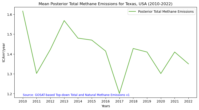
Summary
In this notebook, we have successfully completed the following steps for the GOSAT-based Top-down Total and Natural Methane Emissions dataset:
- Install and import the necessary libraries
- Fetch the collection from STAC using the appropriate endpoints
- Count the number of existing files (granules) within the collection
- Map the methane emission levels
- Generate zonal statistics for the area of interest (AOI)
- Plot a time series analysis of mean methane emission levels for a specified region
If you have any questions regarding this user notebook, please contact us using the feedback form.