# Import the following libraries
# For fetching from the Raster API
import requests
# For making maps
import folium
import folium.plugins
from folium import Map, TileLayer
# For talking to the STAC API
from pystac_client import Client
# For working with data
import pandas as pd
# For making time series
import matplotlib.pyplot as plt
# For formatting date/time data
import datetime
# Custom functions for working with GHGC data via the API
import ghgc_utilsVulcan Fossil Fuel CO₂ Emissions
Annual (2010 - 2021), 1 km resolution estimates of carbon dioxide emissions from fossil fuels and cement production over the contiguous United States, version 4.0.
Author
Siddharth Chaudhary, Paridhi Parajuli
Published
August 30, 2024
Access this Notebook
You can launch this notebook in the US GHG Center JupyterHub (requires access) by clicking the following link: Vulcan Fossil Fuel CO₂ Emissions. If you are a new user, you should first sign up for the hub by filling out this request form and providing the required information.
If you do not have a US GHG Center Jupyterhub account, you can access this notebook through MyBinder by clicking the button below.
![]()
Table of Contents
Data Summary and Application
- Spatial coverage: Contiguous United States
- Spatial resolution: 1 km x 1 km
- Temporal extent: 2010 - 2021
- Temporal resolution: Annual
- Unit: Metric tons of carbon dioxide per 1 km x 1 km grid cell per year (tonne CO₂/km²/year)
- Utility: Climate Research
For more information, visit the Vulcan Fossil Fuel CO₂ Emissions data overview page.
Approach
- Identify available dates and temporal frequency of observations for the given collection using the US Greenhouse Gas Center (GHGC) Application Programming Interface (API)
/stacendpoint. The collection processed in this notebook is the Vulcan Fossil Fuel CO₂ Emissions data product. - Pass the STAC item into the raster API
/collections/{collection_id}/items/{item_id}/{tile_matrix_set_id}/tilejson.jsonendpoint. - Using
folium.plugins.DualMap, visualize two tiles (side-by-side), allowing time point comparison. - After the visualization, perform zonal statistics for a given polygon.
- Create a time-series analysis.
About the Data
Vulcan Fossil Fuel CO2 Emissions
The Vulcan version 4.0 data product represents total carbon dioxide (CO₂) emissions resulting from the combustion of fossil fuel (ff) for the contiguous United States and District of Columbia. Referred to as ffCO₂, the emissions from Vulcan are also categorized into 10 source sectors including; airports, cement production, commercial marine vessels, commercial, power plants, industrial, non-road, on-road, residential and railroads. Data are gridded annually on a 1-km grid for the years 2010 to 2021. These data are annual sums of hourly estimates. Shown is the estimated total annual ffCO₂ for the United States, as well as the estimated total annual ffCO₂ per sector.
For more information regarding this dataset, please visit the Vulcan Fossil Fuel CO₂ Emissions data overview page.
Terminology
Navigating data via the GHGC API, you will encounter terminology that is different from browsing in a typical filesystem. We’ll define some terms here which are used throughout this notebook.
catalog: All datasets available at the/stacendpointcollection: A specific dataset, e.g. Vulcan v4.0item: One data file (i.e. granule) in the dataset, e.g. one annual file of fossil fuel CO2 emissionsasset: A variable available within the granule, e.g. CO2 emissions from residential buildings, airports, or cementSTAC API: SpatioTemporal Asset Catalogs - Endpoint for fetching metadata about available datasetsRaster API: Endpoint for fetching data itself, for imagery and statistics
Install the Required Libraries
Required libraries are pre-installed on the US GHG Center Hub. If you need to run this notebook elsewhere, please install them with this line in a code cell:
%pip install requests folium rasterstats pystac_client pandas matplotlib –quiet
Query the STAC API
STAC API Collection Names
Now, you must fetch the dataset from the STAC API by defining its associated STAC API collection ID as a variable. The collection ID, also known as the collection name, for the Vulcan Fossil Fuel CO2 Emissions dataset is vulcan-ffco2-yeargrid-v4.
# Provide STAC and RASTER API endpoints
STAC_API_URL = "https://earth.gov/ghgcenter/api/stac"
RASTER_API_URL = "https://earth.gov/ghgcenter/api/raster"

# Please use the collection name similar to the one used in the STAC collection.
# Name of the collection for Vulcan Fossil Fuel CO₂ Emissions
collection_name = "vulcan-ffco2-yeargrid-v4"
<CollectionClient id=vulcan-ffco2-yeargrid-v4>
- type "Collection"
- id "vulcan-ffco2-yeargrid-v4"
- stac_version "1.1.0"
- description "Annual (2010 - 2021), 1 km resolution estimates of carbon dioxide emissions from fossil fuels and cement production over the contiguous United States, version 4.0"
links[] 5 items
0
- rel "items"
- href "https://earth.gov/ghgcenter/api/stac/collections/vulcan-ffco2-yeargrid-v4/items"
- type "application/geo+json"
1
- rel "parent"
- href "https://earth.gov/ghgcenter/api/stac/"
- type "application/json"
2
- rel "root"
- href "https://earth.gov/ghgcenter/api/stac"
- type "application/json"
- title "US GHG Center STAC API"
3
- rel "self"
- href "https://earth.gov/ghgcenter/api/stac/collections/vulcan-ffco2-yeargrid-v4"
- type "application/json"
4
- rel "http://www.opengis.net/def/rel/ogc/1.0/queryables"
- href "https://earth.gov/ghgcenter/api/stac/collections/vulcan-ffco2-yeargrid-v4/queryables"
- type "application/schema+json"
- title "Queryables"
stac_extensions[] 2 items
- 0 "https://stac-extensions.github.io/render/v1.0.0/schema.json"
- 1 "https://stac-extensions.github.io/item-assets/v1.0.0/schema.json"
renders
air-co2
assets[] 1 items
- 0 "air-co2"
rescale[] 1 items
0[] 2 items
- 0 0
- 1 1400
- colormap_name "spectral_r"
cmt-co2
assets[] 1 items
- 0 "cmt-co2"
rescale[] 1 items
0[] 2 items
- 0 0
- 1 1400
- colormap_name "spectral_r"
cmv-co2
assets[] 1 items
- 0 "cmv-co2"
rescale[] 1 items
0[] 2 items
- 0 0
- 1 1400
- colormap_name "spectral_r"
com-co2
assets[] 1 items
- 0 "com-co2"
rescale[] 1 items
0[] 2 items
- 0 0
- 1 1400
- colormap_name "spectral_r"
elc-co2
assets[] 1 items
- 0 "elc-co2"
rescale[] 1 items
0[] 2 items
- 0 0
- 1 1400
- colormap_name "spectral_r"
ind-co2
assets[] 1 items
- 0 "ind-co2"
rescale[] 1 items
0[] 2 items
- 0 0
- 1 1400
- colormap_name "spectral_r"
nrd-co2
assets[] 1 items
- 0 "nrd-co2"
rescale[] 1 items
0[] 2 items
- 0 0
- 1 1400
- colormap_name "spectral_r"
onr-co2
assets[] 1 items
- 0 "onr-co2"
rescale[] 1 items
0[] 2 items
- 0 0
- 1 1400
- colormap_name "spectral_r"
res-co2
assets[] 1 items
- 0 "res-co2"
rescale[] 1 items
0[] 2 items
- 0 0
- 1 1400
- colormap_name "spectral_r"
rrd-co2
assets[] 1 items
- 0 "rrd-co2"
rescale[] 1 items
0[] 2 items
- 0 0
- 1 1400
- colormap_name "spectral_r"
dashboard
assets[] 1 items
- 0 "total-co2"
rescale[] 1 items
0[] 2 items
- 0 0
- 1 1400
- colormap_name "spectral_r"
total-co2
assets[] 1 items
- 0 "total-co2"
rescale[] 1 items
0[] 2 items
- 0 0
- 1 1400
- colormap_name "spectral_r"
item_assets
cog_default
- type "image/tiff; application=geotiff; profile=cloud-optimized"
roles[] 2 items
- 0 "data"
- 1 "layer"
- title "Default COG Layer"
- description "Cloud optimized default layer to display on map"
- dashboard:is_periodic True
- dashboard:time_density "year"
- title "Vulcan Fossil Fuel CO₂ Emissions v4.0"
extent
spatial
bbox[] 1 items
0[] 4 items
- 0 -128.22655
- 1 47.89015278
- 2 -65.30824167
- 3 22.85824167
temporal
interval[] 1 items
0[] 2 items
- 0 "2011-01-01T00:00:00Z"
- 1 "2021-12-31T00:00:00Z"
- license "CC-BY-NC-4.0"
providers[] 1 items
0
- name "North American Carbon Program"
roles[] 2 items
- 0 "producer"
- 1 "licensor"
- url "https://vulcan.rc.nau.edu/"
Examining the contents of the collection under the temporal variable, we see that the data is available from January 2010 to December 2021. Looking at the dashboard:time density, the data is periodic with year time density.
# Using PySTAC client
# Fetch the collection from the STAC API using the appropriate endpoint
# The 'pystac' library allows a HTTP request possible
catalog = Client.open(STAC_API_URL)
collection = catalog.get_collection(collection_name)

# Print the properties of the collection to the console
collection
<CollectionClient id=vulcan-ffco2-yeargrid-v4>
- type "Collection"
- id "vulcan-ffco2-yeargrid-v4"
- stac_version "1.1.0"
- description "Annual (2010 - 2021), 1 km resolution estimates of carbon dioxide emissions from fossil fuels and cement production over the contiguous United States, version 4.0"
links[] 5 items
0
- rel "items"
- href "https://earth.gov/ghgcenter/api/stac/collections/vulcan-ffco2-yeargrid-v4/items"
- type "application/geo+json"
1
- rel "parent"
- href "https://earth.gov/ghgcenter/api/stac/"
- type "application/json"
2
- rel "root"
- href "https://earth.gov/ghgcenter/api/stac"
- type "application/json"
- title "US GHG Center STAC API"
3
- rel "self"
- href "https://earth.gov/ghgcenter/api/stac/collections/vulcan-ffco2-yeargrid-v4"
- type "application/json"
4
- rel "http://www.opengis.net/def/rel/ogc/1.0/queryables"
- href "https://earth.gov/ghgcenter/api/stac/collections/vulcan-ffco2-yeargrid-v4/queryables"
- type "application/schema+json"
- title "Queryables"
stac_extensions[] 2 items
- 0 "https://stac-extensions.github.io/render/v1.0.0/schema.json"
- 1 "https://stac-extensions.github.io/item-assets/v1.0.0/schema.json"
renders
air-co2
assets[] 1 items
- 0 "air-co2"
rescale[] 1 items
0[] 2 items
- 0 0
- 1 1400
- colormap_name "spectral_r"
cmt-co2
assets[] 1 items
- 0 "cmt-co2"
rescale[] 1 items
0[] 2 items
- 0 0
- 1 1400
- colormap_name "spectral_r"
cmv-co2
assets[] 1 items
- 0 "cmv-co2"
rescale[] 1 items
0[] 2 items
- 0 0
- 1 1400
- colormap_name "spectral_r"
com-co2
assets[] 1 items
- 0 "com-co2"
rescale[] 1 items
0[] 2 items
- 0 0
- 1 1400
- colormap_name "spectral_r"
elc-co2
assets[] 1 items
- 0 "elc-co2"
rescale[] 1 items
0[] 2 items
- 0 0
- 1 1400
- colormap_name "spectral_r"
ind-co2
assets[] 1 items
- 0 "ind-co2"
rescale[] 1 items
0[] 2 items
- 0 0
- 1 1400
- colormap_name "spectral_r"
nrd-co2
assets[] 1 items
- 0 "nrd-co2"
rescale[] 1 items
0[] 2 items
- 0 0
- 1 1400
- colormap_name "spectral_r"
onr-co2
assets[] 1 items
- 0 "onr-co2"
rescale[] 1 items
0[] 2 items
- 0 0
- 1 1400
- colormap_name "spectral_r"
res-co2
assets[] 1 items
- 0 "res-co2"
rescale[] 1 items
0[] 2 items
- 0 0
- 1 1400
- colormap_name "spectral_r"
rrd-co2
assets[] 1 items
- 0 "rrd-co2"
rescale[] 1 items
0[] 2 items
- 0 0
- 1 1400
- colormap_name "spectral_r"
dashboard
assets[] 1 items
- 0 "total-co2"
rescale[] 1 items
0[] 2 items
- 0 0
- 1 1400
- colormap_name "spectral_r"
total-co2
assets[] 1 items
- 0 "total-co2"
rescale[] 1 items
0[] 2 items
- 0 0
- 1 1400
- colormap_name "spectral_r"
item_assets
cog_default
- type "image/tiff; application=geotiff; profile=cloud-optimized"
roles[] 2 items
- 0 "data"
- 1 "layer"
- title "Default COG Layer"
- description "Cloud optimized default layer to display on map"
- dashboard:is_periodic True
- dashboard:time_density "year"
- title "Vulcan Fossil Fuel CO₂ Emissions v4.0"
extent
spatial
bbox[] 1 items
0[] 4 items
- 0 -128.22655
- 1 47.89015278
- 2 -65.30824167
- 3 22.85824167
temporal
interval[] 1 items
0[] 2 items
- 0 "2011-01-01T00:00:00Z"
- 1 "2021-12-31T00:00:00Z"
- license "CC-BY-NC-4.0"
providers[] 1 items
0
- name "North American Carbon Program"
roles[] 2 items
- 0 "producer"
- 1 "licensor"
- url "https://vulcan.rc.nau.edu/"
# Fetch items directly using search instead of get_items() to avoid the href error
# The collection has an asset without an 'href' field which causes get_items() to fail
search = catalog.search(
    collections=[collection_name],
    max_items=None
)

# Get items as dictionaries first
items_dicts = list(search.items_as_dicts())

# Remove the problematic 'cog_default' asset that's missing 'href' field
for item_dict in items_dicts:
    if 'cog_default' in item_dict.get('assets', {}):
        del item_dict['assets']['cog_default']

# Convert to proper Item objects
from pystac import Item
items = [Item.from_dict(item_dict) for item_dict in items_dicts]

print(f"Found {len(items)} items")
items
Found 12 items[<Item id=vulcan-ffco2-yeargrid-v4-2021>,
<Item id=vulcan-ffco2-yeargrid-v4-2020>,
<Item id=vulcan-ffco2-yeargrid-v4-2019>,
<Item id=vulcan-ffco2-yeargrid-v4-2018>,
<Item id=vulcan-ffco2-yeargrid-v4-2017>,
<Item id=vulcan-ffco2-yeargrid-v4-2016>,
<Item id=vulcan-ffco2-yeargrid-v4-2015>,
<Item id=vulcan-ffco2-yeargrid-v4-2014>,
<Item id=vulcan-ffco2-yeargrid-v4-2013>,
<Item id=vulcan-ffco2-yeargrid-v4-2012>,
<Item id=vulcan-ffco2-yeargrid-v4-2011>,
<Item id=vulcan-ffco2-yeargrid-v4-2010>]
<Item id=vulcan-ffco2-yeargrid-v4-2021>
- type "Feature"
- stac_version "1.1.0"
stac_extensions[] 2 items
- 0 "https://stac-extensions.github.io/raster/v1.1.0/schema.json"
- 1 "https://stac-extensions.github.io/projection/v2.0.0/schema.json"
- id "vulcan-ffco2-yeargrid-v4-2021"
geometry
- type "Polygon"
coordinates[] 1 items
0[] 5 items
0[] 2 items
- 0 -128.22654896758996
- 1 22.857766529124284
1[] 2 items
- 0 -65.30917199495289
- 1 22.857766529124284
2[] 2 items
- 0 -65.30917199495289
- 1 51.44087947724907
3[] 2 items
- 0 -128.22654896758996
- 1 51.44087947724907
4[] 2 items
- 0 -128.22654896758996
- 1 22.857766529124284
bbox[] 4 items
- 0 -128.22654896758996
- 1 22.857766529124284
- 2 -65.30917199495289
- 3 51.44087947724907
properties
- end_datetime "2021-12-31T00:00:00+00:00"
- start_datetime "2021-01-01T00:00:00+00:00"
- datetime None
links[] 5 items
0
- rel "collection"
- href "https://earth.gov/ghgcenter/api/stac/collections/vulcan-ffco2-yeargrid-v4"
- type "application/json"
1
- rel "parent"
- href "https://earth.gov/ghgcenter/api/stac/collections/vulcan-ffco2-yeargrid-v4"
- type "application/json"
2
- rel "root"
- href "https://earth.gov/ghgcenter/api/stac/"
- type "application/json"
3
- rel "self"
- href "https://earth.gov/ghgcenter/api/stac/collections/vulcan-ffco2-yeargrid-v4/items/vulcan-ffco2-yeargrid-v4-2021"
- type "application/geo+json"
4
- rel "preview"
- href "https://earth.gov/ghgcenter/api/raster/collections/vulcan-ffco2-yeargrid-v4/items/vulcan-ffco2-yeargrid-v4-2021/WebMercatorQuad/map?assets=total-co2&rescale=0%2C1400&colormap_name=spectral_r"
- type "text/html"
- title "Map of Item"
assets
air-co2
- href "s3://ghgc-data-store/vulcan-ffco2-yeargrid-v4/AIR_CO2_USA_mosaic_grid_1km_mn_2021.tif"
- type "image/tiff; application=geotiff"
- title "Total Airport CO₂ Emissions"
proj:bbox[] 4 items
- 0 -128.22654896758996
- 1 22.857766529124284
- 2 -65.30917199495289
- 3 51.44087947724907
- proj:wkt2 "GEOGCS["WGS 84",DATUM["WGS_1984",SPHEROID["WGS 84",6378137,298.257223563,AUTHORITY["EPSG","7030"]],AUTHORITY["EPSG","6326"]],PRIMEM["Greenwich",0,AUTHORITY["EPSG","8901"]],UNIT["degree",0.0174532925199433,AUTHORITY["EPSG","9122"]],AXIS["Latitude",NORTH],AXIS["Longitude",EAST],AUTHORITY["EPSG","4326"]]"
proj:shape[] 2 items
- 0 2649
- 1 5831
raster:bands[] 1 items
0
- scale 1.0
- nodata -9999.0
- offset 0.0
- sampling "area"
- data_type "float32"
histogram
- max 318726.1875
- min 0.11889950931072235
- count 11
buckets[] 10 items
- 0 14659
- 1 40
- 2 6
- 3 2
- 4 4
- 5 0
- 6 2
- 7 0
- 8 0
- 9 1
statistics
- mean 1190.7966562457523
- stddev 5906.230747537605
- maximum 318726.1875
- minimum 0.11889950931072235
- valid_percent 3.083506571888412
proj:geometry
- type "Polygon"
coordinates[] 1 items
0[] 5 items
0[] 2 items
- 0 -128.22654896758996
- 1 22.857766529124284
1[] 2 items
- 0 -65.30917199495289
- 1 22.857766529124284
2[] 2 items
- 0 -65.30917199495289
- 1 51.44087947724907
3[] 2 items
- 0 -128.22654896758996
- 1 51.44087947724907
4[] 2 items
- 0 -128.22654896758996
- 1 22.857766529124284
proj:projjson
id
- code 4326
- authority "EPSG"
- name "WGS 84"
- type "GeographicCRS"
datum
- name "World Geodetic System 1984"
- type "GeodeticReferenceFrame"
ellipsoid
- name "WGS 84"
- semi_major_axis 6378137
- inverse_flattening 298.257223563
- $schema "https://proj.org/schemas/v0.7/projjson.schema.json"
coordinate_system
axis[] 2 items
0
- name "Geodetic latitude"
- unit "degree"
- direction "north"
- abbreviation "Lat"
1
- name "Geodetic longitude"
- unit "degree"
- direction "east"
- abbreviation "Lon"
- subtype "ellipsoidal"
proj:transform[] 9 items
- 0 0.01079015211329739
- 1 0.0
- 2 -128.22654896758996
- 3 0.0
- 4 -0.01079015211329739
- 5 51.44087947724907
- 6 0.0
- 7 0.0
- 8 1.0
- proj:code "EPSG:4326"
cmt-co2
- href "s3://ghgc-data-store/vulcan-ffco2-yeargrid-v4/CMT_CO2_USA_mosaic_grid_1km_mn_2021.tif"
- type "image/tiff; application=geotiff"
- title "Total Cement CO₂ Emissions"
proj:bbox[] 4 items
- 0 -128.22654896758996
- 1 22.857766529124284
- 2 -65.30917199495289
- 3 51.44087947724907
- proj:wkt2 "GEOGCS["WGS 84",DATUM["WGS_1984",SPHEROID["WGS 84",6378137,298.257223563,AUTHORITY["EPSG","7030"]],AUTHORITY["EPSG","6326"]],PRIMEM["Greenwich",0,AUTHORITY["EPSG","8901"]],UNIT["degree",0.0174532925199433,AUTHORITY["EPSG","9122"]],AXIS["Latitude",NORTH],AXIS["Longitude",EAST],AUTHORITY["EPSG","4326"]]"
proj:shape[] 2 items
- 0 2649
- 1 5831
raster:bands[] 1 items
0
- scale 1.0
- nodata -9999.0
- offset 0.0
- sampling "area"
- data_type "float32"
histogram
- max 538037.5
- min 14599.9677734375
- count 11
buckets[] 10 items
- 0 10
- 1 15
- 2 19
- 3 7
- 4 9
- 5 4
- 6 4
- 7 6
- 8 0
- 9 1
statistics
- mean 181749.84
- stddev 114981.70564725697
- maximum 538037.5
- minimum 14599.9677734375
- valid_percent 0.015717207618025753
proj:geometry
- type "Polygon"
coordinates[] 1 items
0[] 5 items
0[] 2 items
- 0 -128.22654896758996
- 1 22.857766529124284
1[] 2 items
- 0 -65.30917199495289
- 1 22.857766529124284
2[] 2 items
- 0 -65.30917199495289
- 1 51.44087947724907
3[] 2 items
- 0 -128.22654896758996
- 1 51.44087947724907
4[] 2 items
- 0 -128.22654896758996
- 1 22.857766529124284
proj:projjson
id
- code 4326
- authority "EPSG"
- name "WGS 84"
- type "GeographicCRS"
datum
- name "World Geodetic System 1984"
- type "GeodeticReferenceFrame"
ellipsoid
- name "WGS 84"
- semi_major_axis 6378137
- inverse_flattening 298.257223563
- $schema "https://proj.org/schemas/v0.7/projjson.schema.json"
coordinate_system
axis[] 2 items
0
- name "Geodetic latitude"
- unit "degree"
- direction "north"
- abbreviation "Lat"
1
- name "Geodetic longitude"
- unit "degree"
- direction "east"
- abbreviation "Lon"
- subtype "ellipsoidal"
proj:transform[] 9 items
- 0 0.01079015211329739
- 1 0.0
- 2 -128.22654896758996
- 3 0.0
- 4 -0.01079015211329739
- 5 51.44087947724907
- 6 0.0
- 7 0.0
- 8 1.0
- proj:code "EPSG:4326"
cmv-co2
- href "s3://ghgc-data-store/vulcan-ffco2-yeargrid-v4/CMV_CO2_USA_mosaic_grid_1km_mn_2021.tif"
- type "image/tiff; application=geotiff"
- title "Total Commercial Marine Vessels CO₂ Emissions"
proj:bbox[] 4 items
- 0 -128.22654896758996
- 1 22.857766529124284
- 2 -65.30917199495289
- 3 51.44087947724907
- proj:wkt2 "GEOGCS["WGS 84",DATUM["WGS_1984",SPHEROID["WGS 84",6378137,298.257223563,AUTHORITY["EPSG","7030"]],AUTHORITY["EPSG","6326"]],PRIMEM["Greenwich",0,AUTHORITY["EPSG","8901"]],UNIT["degree",0.0174532925199433,AUTHORITY["EPSG","9122"]],AXIS["Latitude",NORTH],AXIS["Longitude",EAST],AUTHORITY["EPSG","4326"]]"
proj:shape[] 2 items
- 0 2649
- 1 5831
raster:bands[] 1 items
0
- scale 1.0
- nodata -9999.0
- offset 0.0
- sampling "area"
- data_type "float32"
histogram
- max 15446.8408203125
- min 8.111214810924139e-07
- count 11
buckets[] 10 items
- 0 17370
- 1 16
- 2 5
- 3 1
- 4 2
- 5 0
- 6 1
- 7 0
- 8 0
- 9 1
statistics
- mean 32.60311997010807
- stddev 210.77205857399764
- maximum 15446.8408203125
- minimum 8.111214810924139e-07
- valid_percent 3.6455539163090127
proj:geometry
- type "Polygon"
coordinates[] 1 items
0[] 5 items
0[] 2 items
- 0 -128.22654896758996
- 1 22.857766529124284
1[] 2 items
- 0 -65.30917199495289
- 1 22.857766529124284
2[] 2 items
- 0 -65.30917199495289
- 1 51.44087947724907
3[] 2 items
- 0 -128.22654896758996
- 1 51.44087947724907
4[] 2 items
- 0 -128.22654896758996
- 1 22.857766529124284
proj:projjson
id
- code 4326
- authority "EPSG"
- name "WGS 84"
- type "GeographicCRS"
datum
- name "World Geodetic System 1984"
- type "GeodeticReferenceFrame"
ellipsoid
- name "WGS 84"
- semi_major_axis 6378137
- inverse_flattening 298.257223563
- $schema "https://proj.org/schemas/v0.7/projjson.schema.json"
coordinate_system
axis[] 2 items
0
- name "Geodetic latitude"
- unit "degree"
- direction "north"
- abbreviation "Lat"
1
- name "Geodetic longitude"
- unit "degree"
- direction "east"
- abbreviation "Lon"
- subtype "ellipsoidal"
proj:transform[] 9 items
- 0 0.01079015211329739
- 1 0.0
- 2 -128.22654896758996
- 3 0.0
- 4 -0.01079015211329739
- 5 51.44087947724907
- 6 0.0
- 7 0.0
- 8 1.0
- proj:code "EPSG:4326"
com-co2
- href "s3://ghgc-data-store/vulcan-ffco2-yeargrid-v4/COM_CO2_USA_mosaic_grid_1km_mn_2021.tif"
- type "image/tiff; application=geotiff"
- title "Total Commercial CO₂ Emissions"
proj:bbox[] 4 items
- 0 -128.22654896758996
- 1 22.857766529124284
- 2 -65.30917199495289
- 3 51.44087947724907
- proj:wkt2 "GEOGCS["WGS 84",DATUM["WGS_1984",SPHEROID["WGS 84",6378137,298.257223563,AUTHORITY["EPSG","7030"]],AUTHORITY["EPSG","6326"]],PRIMEM["Greenwich",0,AUTHORITY["EPSG","8901"]],UNIT["degree",0.0174532925199433,AUTHORITY["EPSG","9122"]],AXIS["Latitude",NORTH],AXIS["Longitude",EAST],AUTHORITY["EPSG","4326"]]"
proj:shape[] 2 items
- 0 2649
- 1 5831
raster:bands[] 1 items
0
- scale 1.0
- nodata -9999.0
- offset 0.0
- sampling "area"
- data_type "float32"
histogram
- max 41811.0625
- min 6.441725486361349e-10
- count 11
buckets[] 10 items
- 0 178117
- 1 7
- 2 1
- 3 1
- 4 0
- 5 0
- 6 1
- 7 0
- 8 0
- 9 2
statistics
- mean 10.866918777964285
- stddev 175.08472372009805
- maximum 41811.0625
- minimum 6.441725486361349e-10
- valid_percent 37.32920634388412
proj:geometry
- type "Polygon"
coordinates[] 1 items
0[] 5 items
0[] 2 items
- 0 -128.22654896758996
- 1 22.857766529124284
1[] 2 items
- 0 -65.30917199495289
- 1 22.857766529124284
2[] 2 items
- 0 -65.30917199495289
- 1 51.44087947724907
3[] 2 items
- 0 -128.22654896758996
- 1 51.44087947724907
4[] 2 items
- 0 -128.22654896758996
- 1 22.857766529124284
proj:projjson
id
- code 4326
- authority "EPSG"
- name "WGS 84"
- type "GeographicCRS"
datum
- name "World Geodetic System 1984"
- type "GeodeticReferenceFrame"
ellipsoid
- name "WGS 84"
- semi_major_axis 6378137
- inverse_flattening 298.257223563
- $schema "https://proj.org/schemas/v0.7/projjson.schema.json"
coordinate_system
axis[] 2 items
0
- name "Geodetic latitude"
- unit "degree"
- direction "north"
- abbreviation "Lat"
1
- name "Geodetic longitude"
- unit "degree"
- direction "east"
- abbreviation "Lon"
- subtype "ellipsoidal"
proj:transform[] 9 items
- 0 0.01079015211329739
- 1 0.0
- 2 -128.22654896758996
- 3 0.0
- 4 -0.01079015211329739
- 5 51.44087947724907
- 6 0.0
- 7 0.0
- 8 1.0
- proj:code "EPSG:4326"
elc-co2
- href "s3://ghgc-data-store/vulcan-ffco2-yeargrid-v4/ELC_CO2_USA_mosaic_grid_1km_mn_2021.tif"
- type "image/tiff; application=geotiff"
- title "Total Powerplants CO₂ Emissions"
proj:bbox[] 4 items
- 0 -128.22654896758996
- 1 22.857766529124284
- 2 -65.30917199495289
- 3 51.44087947724907
- proj:wkt2 "GEOGCS["WGS 84",DATUM["WGS_1984",SPHEROID["WGS 84",6378137,298.257223563,AUTHORITY["EPSG","7030"]],AUTHORITY["EPSG","6326"]],PRIMEM["Greenwich",0,AUTHORITY["EPSG","8901"]],UNIT["degree",0.0174532925199433,AUTHORITY["EPSG","9122"]],AXIS["Latitude",NORTH],AXIS["Longitude",EAST],AUTHORITY["EPSG","4326"]]"
proj:shape[] 2 items
- 0 2649
- 1 5831
raster:bands[] 1 items
0
- scale 1.0
- nodata -9999.0
- offset 0.0
- sampling "area"
- data_type "float32"
histogram
- max 5685384.0
- min 1.3666567610925995e-05
- count 11
buckets[] 10 items
- 0 3813
- 1 90
- 2 29
- 3 26
- 4 8
- 5 8
- 6 6
- 7 2
- 8 0
- 9 1
statistics
- mean 94311.64850615115
- stddev 355198.87374596845
- maximum 5685384.0
- minimum 1.3666567610925995e-05
- valid_percent 0.8346885059012876
proj:geometry
- type "Polygon"
coordinates[] 1 items
0[] 5 items
0[] 2 items
- 0 -128.22654896758996
- 1 22.857766529124284
1[] 2 items
- 0 -65.30917199495289
- 1 22.857766529124284
2[] 2 items
- 0 -65.30917199495289
- 1 51.44087947724907
3[] 2 items
- 0 -128.22654896758996
- 1 51.44087947724907
4[] 2 items
- 0 -128.22654896758996
- 1 22.857766529124284
proj:projjson
id
- code 4326
- authority "EPSG"
- name "WGS 84"
- type "GeographicCRS"
datum
- name "World Geodetic System 1984"
- type "GeodeticReferenceFrame"
ellipsoid
- name "WGS 84"
- semi_major_axis 6378137
- inverse_flattening 298.257223563
- $schema "https://proj.org/schemas/v0.7/projjson.schema.json"
coordinate_system
axis[] 2 items
0
- name "Geodetic latitude"
- unit "degree"
- direction "north"
- abbreviation "Lat"
1
- name "Geodetic longitude"
- unit "degree"
- direction "east"
- abbreviation "Lon"
- subtype "ellipsoidal"
proj:transform[] 9 items
- 0 0.01079015211329739
- 1 0.0
- 2 -128.22654896758996
- 3 0.0
- 4 -0.01079015211329739
- 5 51.44087947724907
- 6 0.0
- 7 0.0
- 8 1.0
- proj:code "EPSG:4326"
ind-co2
- href "s3://ghgc-data-store/vulcan-ffco2-yeargrid-v4/IND_CO2_USA_mosaic_grid_1km_mn_2021.tif"
- type "image/tiff; application=geotiff"
- title "Total Industrial CO₂ Emissions"
proj:bbox[] 4 items
- 0 -128.22654896758996
- 1 22.857766529124284
- 2 -65.30917199495289
- 3 51.44087947724907
- proj:wkt2 "GEOGCS["WGS 84",DATUM["WGS_1984",SPHEROID["WGS 84",6378137,298.257223563,AUTHORITY["EPSG","7030"]],AUTHORITY["EPSG","6326"]],PRIMEM["Greenwich",0,AUTHORITY["EPSG","8901"]],UNIT["degree",0.0174532925199433,AUTHORITY["EPSG","9122"]],AXIS["Latitude",NORTH],AXIS["Longitude",EAST],AUTHORITY["EPSG","4326"]]"
proj:shape[] 2 items
- 0 2649
- 1 5831
raster:bands[] 1 items
0
- scale 1.0
- nodata -9999.0
- offset 0.0
- sampling "area"
- data_type "float32"
histogram
- max 3248811.0
- min 7.467048507292517e-11
- count 11
buckets[] 10 items
- 0 110441
- 1 0
- 2 0
- 3 0
- 4 0
- 5 0
- 6 0
- 7 0
- 8 0
- 9 1
statistics
- mean 120.20799152496333
- stddev 9843.60430747931
- maximum 3248811.0
- minimum 7.467048507292517e-11
- valid_percent 23.14453125
proj:geometry
- type "Polygon"
coordinates[] 1 items
0[] 5 items
0[] 2 items
- 0 -128.22654896758996
- 1 22.857766529124284
1[] 2 items
- 0 -65.30917199495289
- 1 22.857766529124284
2[] 2 items
- 0 -65.30917199495289
- 1 51.44087947724907
3[] 2 items
- 0 -128.22654896758996
- 1 51.44087947724907
4[] 2 items
- 0 -128.22654896758996
- 1 22.857766529124284
proj:projjson
id
- code 4326
- authority "EPSG"
- name "WGS 84"
- type "GeographicCRS"
datum
- name "World Geodetic System 1984"
- type "GeodeticReferenceFrame"
ellipsoid
- name "WGS 84"
- semi_major_axis 6378137
- inverse_flattening 298.257223563
- $schema "https://proj.org/schemas/v0.7/projjson.schema.json"
coordinate_system
axis[] 2 items
0
- name "Geodetic latitude"
- unit "degree"
- direction "north"
- abbreviation "Lat"
1
- name "Geodetic longitude"
- unit "degree"
- direction "east"
- abbreviation "Lon"
- subtype "ellipsoidal"
proj:transform[] 9 items
- 0 0.01079015211329739
- 1 0.0
- 2 -128.22654896758996
- 3 0.0
- 4 -0.01079015211329739
- 5 51.44087947724907
- 6 0.0
- 7 0.0
- 8 1.0
- proj:code "EPSG:4326"
nrd-co2
- href "s3://ghgc-data-store/vulcan-ffco2-yeargrid-v4/NRD_CO2_USA_mosaic_grid_1km_mn_2021.tif"
- type "image/tiff; application=geotiff"
- title "Total Nonroad CO₂ Emissions"
proj:bbox[] 4 items
- 0 -128.22654896758996
- 1 22.857766529124284
- 2 -65.30917199495289
- 3 51.44087947724907
- proj:wkt2 "GEOGCS["WGS 84",DATUM["WGS_1984",SPHEROID["WGS 84",6378137,298.257223563,AUTHORITY["EPSG","7030"]],AUTHORITY["EPSG","6326"]],PRIMEM["Greenwich",0,AUTHORITY["EPSG","8901"]],UNIT["degree",0.0174532925199433,AUTHORITY["EPSG","9122"]],AXIS["Latitude",NORTH],AXIS["Longitude",EAST],AUTHORITY["EPSG","4326"]]"
proj:shape[] 2 items
- 0 2649
- 1 5831
raster:bands[] 1 items
0
- scale 1.0
- nodata -9999.0
- offset 0.0
- sampling "area"
- data_type "float32"
histogram
- max 2277.109619140625
- min 1.7788032380394725e-07
- count 11
buckets[] 10 items
- 0 227435
- 1 26
- 2 5
- 3 1
- 4 0
- 5 1
- 6 1
- 7 0
- 8 0
- 9 2
statistics
- mean 6.1029197128425166
- stddev 14.197089191407585
- maximum 2277.109619140625
- minimum 1.7788032380394725e-07
- valid_percent 47.66945245439914
proj:geometry
- type "Polygon"
coordinates[] 1 items
0[] 5 items
0[] 2 items
- 0 -128.22654896758996
- 1 22.857766529124284
1[] 2 items
- 0 -65.30917199495289
- 1 22.857766529124284
2[] 2 items
- 0 -65.30917199495289
- 1 51.44087947724907
3[] 2 items
- 0 -128.22654896758996
- 1 51.44087947724907
4[] 2 items
- 0 -128.22654896758996
- 1 22.857766529124284
proj:projjson
id
- code 4326
- authority "EPSG"
- name "WGS 84"
- type "GeographicCRS"
datum
- name "World Geodetic System 1984"
- type "GeodeticReferenceFrame"
ellipsoid
- name "WGS 84"
- semi_major_axis 6378137
- inverse_flattening 298.257223563
- $schema "https://proj.org/schemas/v0.7/projjson.schema.json"
coordinate_system
axis[] 2 items
0
- name "Geodetic latitude"
- unit "degree"
- direction "north"
- abbreviation "Lat"
1
- name "Geodetic longitude"
- unit "degree"
- direction "east"
- abbreviation "Lon"
- subtype "ellipsoidal"
proj:transform[] 9 items
- 0 0.01079015211329739
- 1 0.0
- 2 -128.22654896758996
- 3 0.0
- 4 -0.01079015211329739
- 5 51.44087947724907
- 6 0.0
- 7 0.0
- 8 1.0
- proj:code "EPSG:4326"
onr-co2
- href "s3://ghgc-data-store/vulcan-ffco2-yeargrid-v4/ONR_CO2_USA_mosaic_grid_1km_mn_2021.tif"
- type "image/tiff; application=geotiff"
- title "Total Onroad CO₂ Emissions"
proj:bbox[] 4 items
- 0 -128.22654896758996
- 1 22.857766529124284
- 2 -65.30917199495289
- 3 51.44087947724907
- proj:wkt2 "GEOGCS["WGS 84",DATUM["WGS_1984",SPHEROID["WGS 84",6378137,298.257223563,AUTHORITY["EPSG","7030"]],AUTHORITY["EPSG","6326"]],PRIMEM["Greenwich",0,AUTHORITY["EPSG","8901"]],UNIT["degree",0.0174532925199433,AUTHORITY["EPSG","9122"]],AXIS["Latitude",NORTH],AXIS["Longitude",EAST],AUTHORITY["EPSG","4326"]]"
proj:shape[] 2 items
- 0 2649
- 1 5831
raster:bands[] 1 items
0
- scale 1.0
- nodata -9999.0
- offset 0.0
- sampling "area"
- data_type "float32"
histogram
- max 16120.27734375
- min 0.0011055185459554195
- count 11
buckets[] 10 items
- 0 195583
- 1 803
- 2 88
- 3 22
- 4 3
- 5 2
- 6 0
- 7 0
- 8 0
- 9 1
statistics
- mean 64.57338856601969
- stddev 230.03362908149538
- maximum 16120.27734375
- minimum 0.0011055185459554195
- valid_percent 41.179503084763944
proj:geometry
- type "Polygon"
coordinates[] 1 items
0[] 5 items
0[] 2 items
- 0 -128.22654896758996
- 1 22.857766529124284
1[] 2 items
- 0 -65.30917199495289
- 1 22.857766529124284
2[] 2 items
- 0 -65.30917199495289
- 1 51.44087947724907
3[] 2 items
- 0 -128.22654896758996
- 1 51.44087947724907
4[] 2 items
- 0 -128.22654896758996
- 1 22.857766529124284
proj:projjson
id
- code 4326
- authority "EPSG"
- name "WGS 84"
- type "GeographicCRS"
datum
- name "World Geodetic System 1984"
- type "GeodeticReferenceFrame"
ellipsoid
- name "WGS 84"
- semi_major_axis 6378137
- inverse_flattening 298.257223563
- $schema "https://proj.org/schemas/v0.7/projjson.schema.json"
coordinate_system
axis[] 2 items
0
- name "Geodetic latitude"
- unit "degree"
- direction "north"
- abbreviation "Lat"
1
- name "Geodetic longitude"
- unit "degree"
- direction "east"
- abbreviation "Lon"
- subtype "ellipsoidal"
proj:transform[] 9 items
- 0 0.01079015211329739
- 1 0.0
- 2 -128.22654896758996
- 3 0.0
- 4 -0.01079015211329739
- 5 51.44087947724907
- 6 0.0
- 7 0.0
- 8 1.0
- proj:code "EPSG:4326"
res-co2
- href "s3://ghgc-data-store/vulcan-ffco2-yeargrid-v4/RES_CO2_USA_mosaic_grid_1km_mn_2021.tif"
- type "image/tiff; application=geotiff"
- title "Total Residential CO₂ Emissions"
proj:bbox[] 4 items
- 0 -128.22654896758996
- 1 22.857766529124284
- 2 -65.30917199495289
- 3 51.44087947724907
- proj:wkt2 "GEOGCS["WGS 84",DATUM["WGS_1984",SPHEROID["WGS 84",6378137,298.257223563,AUTHORITY["EPSG","7030"]],AUTHORITY["EPSG","6326"]],PRIMEM["Greenwich",0,AUTHORITY["EPSG","8901"]],UNIT["degree",0.0174532925199433,AUTHORITY["EPSG","9122"]],AXIS["Latitude",NORTH],AXIS["Longitude",EAST],AUTHORITY["EPSG","4326"]]"
proj:shape[] 2 items
- 0 2649
- 1 5831
raster:bands[] 1 items
0
- scale 1.0
- nodata -9999.0
- offset 0.0
- sampling "area"
- data_type "float32"
histogram
- max 10387.0556640625
- min 9.804268508162295e-09
- count 11
buckets[] 10 items
- 0 204532
- 1 112
- 2 28
- 3 7
- 4 4
- 5 3
- 6 3
- 7 2
- 8 1
- 9 1
statistics
- mean 12.793920651903093
- stddev 91.07716732362586
- maximum 10387.0556640625
- minimum 9.804268508162295e-09
- valid_percent 42.896031719420606
proj:geometry
- type "Polygon"
coordinates[] 1 items
0[] 5 items
0[] 2 items
- 0 -128.22654896758996
- 1 22.857766529124284
1[] 2 items
- 0 -65.30917199495289
- 1 22.857766529124284
2[] 2 items
- 0 -65.30917199495289
- 1 51.44087947724907
3[] 2 items
- 0 -128.22654896758996
- 1 51.44087947724907
4[] 2 items
- 0 -128.22654896758996
- 1 22.857766529124284
proj:projjson
id
- code 4326
- authority "EPSG"
- name "WGS 84"
- type "GeographicCRS"
datum
- name "World Geodetic System 1984"
- type "GeodeticReferenceFrame"
ellipsoid
- name "WGS 84"
- semi_major_axis 6378137
- inverse_flattening 298.257223563
- $schema "https://proj.org/schemas/v0.7/projjson.schema.json"
coordinate_system
axis[] 2 items
0
- name "Geodetic latitude"
- unit "degree"
- direction "north"
- abbreviation "Lat"
1
- name "Geodetic longitude"
- unit "degree"
- direction "east"
- abbreviation "Lon"
- subtype "ellipsoidal"
proj:transform[] 9 items
- 0 0.01079015211329739
- 1 0.0
- 2 -128.22654896758996
- 3 0.0
- 4 -0.01079015211329739
- 5 51.44087947724907
- 6 0.0
- 7 0.0
- 8 1.0
- proj:code "EPSG:4326"
rrd-co2
- href "s3://ghgc-data-store/vulcan-ffco2-yeargrid-v4/RRD_CO2_USA_mosaic_grid_1km_mn_2021.tif"
- type "image/tiff; application=geotiff"
- title "Total Railroad CO₂ Emissions"
- description "Estimated total annual ffCO₂ emissions coming from railroads."
proj:bbox[] 4 items
- 0 -128.22654896758996
- 1 22.857766529124284
- 2 -65.30917199495289
- 3 51.44087947724907
- proj:wkt2 "GEOGCS["WGS 84",DATUM["WGS_1984",SPHEROID["WGS 84",6378137,298.257223563,AUTHORITY["EPSG","7030"]],AUTHORITY["EPSG","6326"]],PRIMEM["Greenwich",0,AUTHORITY["EPSG","8901"]],UNIT["degree",0.0174532925199433,AUTHORITY["EPSG","9122"]],AXIS["Latitude",NORTH],AXIS["Longitude",EAST],AUTHORITY["EPSG","4326"]]"
proj:shape[] 2 items
- 0 2649
- 1 5831
raster:bands[] 1 items
0
- scale 1.0
- nodata -9999.0
- offset 0.0
- sampling "area"
- data_type "float32"
histogram
- max 4935.501953125
- min 7.793863915139809e-05
- count 11
buckets[] 10 items
- 0 43982
- 1 167
- 2 38
- 3 9
- 4 7
- 5 5
- 6 3
- 7 2
- 8 1
- 9 2
statistics
- mean 24.959290754478015
- stddev 94.2219837346061
- maximum 4935.501953125
- minimum 7.793863915139809e-05
- valid_percent 9.266027360515022
proj:geometry
- type "Polygon"
coordinates[] 1 items
0[] 5 items
0[] 2 items
- 0 -128.22654896758996
- 1 22.857766529124284
1[] 2 items
- 0 -65.30917199495289
- 1 22.857766529124284
2[] 2 items
- 0 -65.30917199495289
- 1 51.44087947724907
3[] 2 items
- 0 -128.22654896758996
- 1 51.44087947724907
4[] 2 items
- 0 -128.22654896758996
- 1 22.857766529124284
proj:projjson
id
- code 4326
- authority "EPSG"
- name "WGS 84"
- type "GeographicCRS"
datum
- name "World Geodetic System 1984"
- type "GeodeticReferenceFrame"
ellipsoid
- name "WGS 84"
- semi_major_axis 6378137
- inverse_flattening 298.257223563
- $schema "https://proj.org/schemas/v0.7/projjson.schema.json"
coordinate_system
axis[] 2 items
0
- name "Geodetic latitude"
- unit "degree"
- direction "north"
- abbreviation "Lat"
1
- name "Geodetic longitude"
- unit "degree"
- direction "east"
- abbreviation "Lon"
- subtype "ellipsoidal"
proj:transform[] 9 items
- 0 0.01079015211329739
- 1 0.0
- 2 -128.22654896758996
- 3 0.0
- 4 -0.01079015211329739
- 5 51.44087947724907
- 6 0.0
- 7 0.0
- 8 1.0
- proj:code "EPSG:4326"
total-co2
- href "s3://ghgc-data-store/vulcan-ffco2-yeargrid-v4/TOT_CO2_USA_mosaic_grid_1km_mn_2021.tif"
- type "image/tiff; application=geotiff"
- title "Total of all sectors CO₂ Emissions"
- description "Estimated total annual CO₂ emissions from fossil fuel combustion (ffCO₂) across all sectors."
proj:bbox[] 4 items
- 0 -128.22654896758996
- 1 22.857766529124284
- 2 -65.30917199495289
- 3 51.44087947724907
- proj:wkt2 "GEOGCS["WGS 84",DATUM["WGS_1984",SPHEROID["WGS 84",6378137,298.257223563,AUTHORITY["EPSG","7030"]],AUTHORITY["EPSG","6326"]],PRIMEM["Greenwich",0,AUTHORITY["EPSG","8901"]],UNIT["degree",0.0174532925199433,AUTHORITY["EPSG","9122"]],AXIS["Latitude",NORTH],AXIS["Longitude",EAST],AUTHORITY["EPSG","4326"]]"
proj:shape[] 2 items
- 0 2649
- 1 5831
raster:bands[] 1 items
0
- scale 1.0
- nodata -9999.0
- offset 0.0
- sampling "area"
- data_type "float32"
histogram
- max 272530.15625
- min 1.7858106104995386e-07
- count 11
buckets[] 10 items
- 0 227843
- 1 81
- 2 36
- 3 7
- 4 3
- 5 6
- 6 1
- 7 4
- 8 1
- 9 1
statistics
- mean 162.91311194255712
- stddev 2080.549384731812
- maximum 272530.15625
- minimum 1.7858106104995386e-07
- valid_percent 47.7767485917382
proj:geometry
- type "Polygon"
coordinates[] 1 items
0[] 5 items
0[] 2 items
- 0 -128.22654896758996
- 1 22.857766529124284
1[] 2 items
- 0 -65.30917199495289
- 1 22.857766529124284
2[] 2 items
- 0 -65.30917199495289
- 1 51.44087947724907
3[] 2 items
- 0 -128.22654896758996
- 1 51.44087947724907
4[] 2 items
- 0 -128.22654896758996
- 1 22.857766529124284
proj:projjson
id
- code 4326
- authority "EPSG"
- name "WGS 84"
- type "GeographicCRS"
datum
- name "World Geodetic System 1984"
- type "GeodeticReferenceFrame"
ellipsoid
- name "WGS 84"
- semi_major_axis 6378137
- inverse_flattening 298.257223563
- $schema "https://proj.org/schemas/v0.7/projjson.schema.json"
coordinate_system
axis[] 2 items
0
- name "Geodetic latitude"
- unit "degree"
- direction "north"
- abbreviation "Lat"
1
- name "Geodetic longitude"
- unit "degree"
- direction "east"
- abbreviation "Lon"
- subtype "ellipsoidal"
proj:transform[] 9 items
- 0 0.01079015211329739
- 1 0.0
- 2 -128.22654896758996
- 3 0.0
- 4 -0.01079015211329739
- 5 51.44087947724907
- 6 0.0
- 7 0.0
- 8 1.0
- proj:code "EPSG:4326"
rendered_preview
- href "https://earth.gov/ghgcenter/api/raster/collections/vulcan-ffco2-yeargrid-v4/items/vulcan-ffco2-yeargrid-v4-2021/preview.png?assets=total-co2&rescale=0%2C1400&colormap_name=spectral_r"
- type "image/png"
- title "Rendered preview"
- rel "preview"
roles[] 1 items
- 0 "overview"
- collection "vulcan-ffco2-yeargrid-v4"
Creating Maps Using Folium
You will now explore changes in CO2 emissions at a given location and time and visualize the outputs on a map using folium.
Fetch Imagery from Raster API
Here we get information from the Raster API, which we will add to our map in the next section.
Below, we use some statistics of the raster data to set upper and lower limits for our color bar. These are saved as the rescale_values, and will be passed to the Raster API in the following step(s).
# Extract collection name and item ID for the first date
first_date = items_dict[dates[0]]
collection_id_1 = first_date.collection_id
item_id_1 = first_date.id

# Select relevant asset
object = first_date.assets[asset_name]
raster_bands = object.extra_fields.get("raster:bands", [{}])

# Print raster bands' information
raster_bands
[{'scale': 1.0,
'nodata': -9999.0,
'offset': 0.0,
'sampling': 'area',
'data_type': 'float32',
'histogram': {'max': 272530.15625,
'min': 1.7858106104995386e-07,
'count': 11,
'buckets': [227843, 81, 36, 7, 3, 6, 1, 4, 1, 1]},
'statistics': {'mean': 162.91311194255712,
'stddev': 2080.549384731812,
'maximum': 272530.15625,
'minimum': 1.7858106104995386e-07,
'valid_percent': 47.7767485917382}}]{'max': 8485.110650869805, 'min': 0.0}Now, you will pass the item id, collection name, asset name, and the rescale values to the Raster API endpoint, along with a colormap. This step is done twice, one for each date/time you will visualize, and tells the Raster API which collection, item, and asset you want to view, specifying the colormap and colorbar ranges to use for visualization. The API returns a JSON with information about the requested image. Each image will be referred to as a tile.
# Make a GET request to retrieve information for the date mentioned above

# Get the S3 URL for the asset
asset_href = first_date.assets[asset_name].href

# Since the standard tilejson endpoint is failing, construct it manually using COG endpoint
print("Using COG tiles endpoint.")

# Get bounds from the item
bbox = first_date.bbox
center_lon = (bbox[0] + bbox[2]) / 2
center_lat = (bbox[1] + bbox[3]) / 2

# Construct tilejson manually using COG tiles endpoint
month1_tile = {
    'tilejson': '2.2.0',
    'name': item_id_1,
    'tiles': [
        f"{RASTER_API_URL}/cog/tiles/WebMercatorQuad/{{z}}/{{x}}/{{y}}"
        f"?url={asset_href}"
        f"&colormap_name={color_map.lower()}"
        f"&rescale={rescale_values['min']},{rescale_values['max']}"
    ],
    'minzoom': 0,
    'maxzoom': 24,
    'bounds': bbox,
    'center': [center_lon, center_lat, 0]
}

# Print the properties of the retrieved granule to the console
month1_tile
Using COG tiles endpoint.{'tilejson': '2.2.0',
'name': 'vulcan-ffco2-yeargrid-v4-2021',
'tiles': ['https://earth.gov/ghgcenter/api/raster/cog/tiles/WebMercatorQuad/{z}/{x}/{y}?url=s3://ghgc-data-store/vulcan-ffco2-yeargrid-v4/TOT_CO2_USA_mosaic_grid_1km_mn_2021.tif&colormap_name=spectral_r&rescale=0.0,8485.110650869805'],
'minzoom': 0,
'maxzoom': 24,
'bounds': [-128.22654896758996,
22.857766529124284,
-65.30917199495289,
51.44087947724907],
'center': [-96.76786048127143, 37.14932300318668, 0]}# Repeat the above for your second date/time
# Note that we do not calculate new rescale_values for this tile
# We want date tiles 1 and 2 to have the same colorbar range for visual comparison
second_date = items_dict[dates[1]]
collection_id_2 = second_date.collection_id
item_id_2 = second_date.id
# Get the S3 URL for the asset
asset_href_2 = second_date.assets[asset_name].href
print("Using COG tiles endpoint.")
# Get bounds from the item
bbox = second_date.bbox
center_lon = (bbox[0] + bbox[2]) / 2
center_lat = (bbox[1] + bbox[3]) / 2
# Construct tilejson manually using COG tiles endpoint
month2_tile = {
'tilejson': '2.2.0',
'name': item_id_2,
'tiles': [
f"{RASTER_API_URL}/cog/tiles/WebMercatorQuad/{{z}}/{{x}}/{{y}}"
f"?url={asset_href_2}"
f"&colormap_name={color_map.lower()}"
f"&rescale={rescale_values['min']},{rescale_values['max']}"
],
'minzoom': 0,
'maxzoom': 24,
'bounds': bbox,
'center': [center_lon, center_lat, 0]
}
# Print the properties of the retrieved granule to the console
month2_tileUsing COG tiles endpoint.{'tilejson': '2.2.0',
'name': 'vulcan-ffco2-yeargrid-v4-2011',
'tiles': ['https://earth.gov/ghgcenter/api/raster/cog/tiles/WebMercatorQuad/{z}/{x}/{y}?url=s3://ghgc-data-store/vulcan-ffco2-yeargrid-v4/TOT_CO2_USA_mosaic_grid_1km_mn_2011.tif&colormap_name=spectral_r&rescale=0.0,8485.110650869805'],
'minzoom': 0,
'maxzoom': 24,
'bounds': [-128.22654896758996,
22.857766529124284,
-65.30917199495289,
51.44087947724907],
'center': [-96.76786048127143, 37.14932300318668, 0]}Generate Map
# Initialize the map, specifying the center of the map and the starting zoom level.
# 'folium.plugins' allows mapping side-by-side via 'DualMap'
# Map is centered on the position specified by "location=(lat,lon)"
map_ = folium.plugins.DualMap(location=(34, -118), zoom_start=6)

# Define the first map layer
map_layer_1 = TileLayer(
    tiles=month1_tile["tiles"][0], # Path to retrieve the tile
    attr="US GHG Center", # Set the attribution
    name=f'{dates[0]} {items[0].assets[asset_name].title}', # Title for the layer
    overlay=True, # The layer can be overlaid on the map
    opacity=0.8, # Adjust the transparency of the layer
)
# Add the first layer to the Dual Map
map_layer_1.add_to(map_.m1)

# Define the second map layer
map_layer_2 = TileLayer(
    tiles=month2_tile["tiles"][0], # Path to retrieve the tile
    attr="US GHG Center", # Set the attribution
    name=f'{dates[1]} {items[0].assets[asset_name].title}', # Title for the layer
    overlay=True, # The layer can be overlaid on the map
    opacity=0.8, # Adjust the transparency of the layer
)
# Add the second layer to the Dual Map
map_layer_2.add_to(map_.m2)

# Add a layer control to switch between map layers
folium.LayerControl(collapsed=False).add_to(map_)

# Add colorbar
# First we'll rescale our numbers to make the labels nicer.
re_rescale_values = {
    "min":rescale_values["min"]/1e3,
    "max":rescale_values["max"]/1e3
}
# We can use 'generate_html_colorbar' from the 'ghgc_utils' module
# to create an HTML colorbar representation.
legend_html = ghgc_utils.generate_html_colorbar(color_map,re_rescale_values,label=f'{items[0].assets[asset_name].title} (10^3 tonne CO₂/km²/year)',dark=True)

# Add colorbar to the map
map_.get_root().html.add_child(folium.Element(legend_html))

map_
Make this Notebook Trusted to load map: File -> Trust Notebook
This map indicates an overall decrease in total CO2 emissions over the Los Angeles, CA basin between 2011 and 2021.
Calculate Zonal Statistics
To perform zonal statistics, first we need to create a polygon. In this use case we are creating a polygon over the Los Angeles, CA basin.
# Give the area of interest (AOI) a name for use in plotting later
aoi_name = "Los Angeles Basin"
# Define AOI as a GeoJSON
aoi = {
    "type": "Feature", # Create a feature object
    "properties": {},
    "geometry": { # Set the bounding coordinates for the polygon
        "coordinates": [
            [
                [-119, 34.34],   # Northwest bounding coordinate
                [-119,33.4],     # Southwest bounding coordinate
                [-117,33.4],     # Southeast bounding coordinate
                [-117,34.34],    # Northeast bounding coordinate
                [-119,34.34]     # Northwest bounding coordinate (closing the polygon)
            ]
        ],
        "type": "Polygon",
    },
}
# Quick Folium map to visualize this AOI
map_ = folium.Map(location=(33.6, -118), zoom_start=8)
# Add AOI to map
folium.GeoJson(aoi, name=aoi_name, style_function=lambda feature: {"fillColor":"none","color":"#FFA1F8"}).add_to(map_)
# Add data layer to visualize number of grid cells within AOI
# (Created in previous section)
map_layer_2.add_to(map_)
# Add a layer control to switch between map layers
folium.LayerControl(collapsed=False).add_to(map_)
# Add a quick colorbar
# (Also utilizes values defined in previous section)
legend_html = ghgc_utils.generate_html_colorbar(color_map,re_rescale_values,label='10^3 tonne CO₂/km²/year',dark=True)
map_.get_root().html.add_child(folium.Element(legend_html))
map_Make this Notebook Trusted to load map: File -> Trust Notebook
We will perform zonal statistics and create a dataframe using our defined AOI for the Los Angeles Basin, the items from our initial catalog search, and the “total-co2” asset.
We can generate the statistics for the AOI using a function from the ghgc_utils module, which fetches the data and its statistics from the Raster API.
Generating stats...
Done!
CPU times: user 616 ms, sys: 30.6 ms, total: 647 ms
Wall time: 9.09 s| datetime | min | max | mean | count | sum | std | median | majority | minority | unique | histogram | valid_percent | masked_pixels | valid_pixels | percentile_2 | percentile_98 | date | |
|---|---|---|---|---|---|---|---|---|---|---|---|---|---|---|---|---|---|---|
| 0 | 2021-01-01T00:00:00+00:00 | 0.02450298517942428589 | 1933603.37500000000000000000 | 5650.57666015625000000000 | 12719.59960937500000000000 | 71873072.00000000000000000000 | 32522.57210000463601318188 | 703.66845703125000000000 | 161.73231506347656250000 | 0.02450298517942428589 | 10873.00000000000000000000 | [[12893, 9, 3, 0, 3, 1, 0, 2, 0, 1], [0.024502... | 78.89000000000000056843 | 3456.00000000000000000000 | 12912.00000000000000000000 | 10.00618267059326171875 | 30891.58203125000000000000 | 2021-01-01 00:00:00+00:00 |
| 1 | 2020-01-01T00:00:00+00:00 | 0.02450298517942428589 | 1960805.00000000000000000000 | 5416.68261718750000000000 | 12719.59960937500000000000 | 68898032.00000000000000000000 | 30049.71028146527896751650 | 677.55438232421875000000 | 146.33135986328125000000 | 0.02450298517942428589 | 10873.00000000000000000000 | [[12893, 11, 2, 2, 1, 1, 0, 1, 0, 1], [0.02450... | 78.89000000000000056843 | 3456.00000000000000000000 | 12912.00000000000000000000 | 9.06154727935791015625 | 29740.44531250000000000000 | 2020-01-01 00:00:00+00:00 |
| 2 | 2019-01-01T00:00:00+00:00 | 0.02285039983689785004 | 1927774.62500000000000000000 | 6158.78076171875000000000 | 12719.59960937500000000000 | 78337224.00000000000000000000 | 30807.42040483104210579768 | 737.57531738281250000000 | 177.19674682617187500000 | 0.02285039983689785004 | 11029.00000000000000000000 | [[12891, 10, 5, 1, 1, 0, 3, 0, 0, 1], [0.02285... | 78.89000000000000056843 | 3456.00000000000000000000 | 12912.00000000000000000000 | 11.07019805908203125000 | 34685.78906250000000000000 | 2019-01-01 00:00:00+00:00 |
| 3 | 2018-01-01T00:00:00+00:00 | 0.03149935230612754822 | 1944060.25000000000000000000 | 6235.81250000000000000000 | 12719.59960937500000000000 | 79317040.00000000000000000000 | 30910.32914739019906846806 | 742.24194335937500000000 | 175.03439331054687500000 | 0.03149935230612754822 | 11028.00000000000000000000 | [[12892, 9, 2, 4, 2, 0, 2, 0, 0, 1], [0.031499... | 78.89000000000000056843 | 3456.00000000000000000000 | 12912.00000000000000000000 | 11.08772563934326171875 | 35405.92187500000000000000 | 2018-01-01 00:00:00+00:00 |
| 4 | 2017-01-01T00:00:00+00:00 | 0.02745403721928596497 | 1941930.87500000000000000000 | 6396.50000000000000000000 | 12719.59960937500000000000 | 81360920.00000000000000000000 | 34066.04784826088143745437 | 747.31213378906250000000 | 175.16557312011718750000 | 0.02745403721928596497 | 11031.00000000000000000000 | [[12891, 10, 2, 3, 1, 1, 2, 0, 1, 1], [0.02745... | 78.89000000000000056843 | 3456.00000000000000000000 | 12912.00000000000000000000 | 11.07795715332031250000 | 35702.85937500000000000000 | 2017-01-01 00:00:00+00:00 |
Time-Series Analysis
We can now explore the total fossil fuel emissions for our AOI. We can plot the data set using the code below:
# Figure size: 10 is width, 5 is height.
fig = plt.figure(figsize=(10,5))
df = df.sort_values(by="datetime")

# Use which_stat to pick any statistic from our DataFrame to visualize
# Change 'which_stat' below if you would rather look at a different statistic, like minimum or maximum
which_stat = "mean"

plt.plot(
    [d[0:4] for d in df["datetime"]], # X-axis: sorted datetime
    df[which_stat], # Y-axis: maximum CO₂
    color="red", # Line color
    linestyle="-", # Line style
    linewidth=2, # Line width,
    marker='o', # Add circle markers at location of data points
    label=f"{which_stat.capitalize()} {items[0].assets[asset_name].title}", # Legend label
)

# Display legend
plt.legend()

# Insert label for the X-axis
plt.xlabel("Year")

# Insert label for the Y-axis
plt.ylabel("tonne C/km²/year")

# Insert title for the plot
plt.title(f"{which_stat.capitalize()} {items[0].assets[asset_name].title} for {aoi_name}")

# Add data citation
plt.text(
    min([d[0:4] for d in df["datetime"]]),           # X-coordinate of the text
    df[which_stat].min(),                  # Y-coordinate of the text
    # Text to be displayed
    f"Source: {collection.title}",      #example text
    fontsize=9,                             # Font size
    horizontalalignment="left",              # Horizontal alignment
    verticalalignment="top",                 # Vertical alignment
    color="blue",                            # Text color
)


# Plot the time series
plt.show()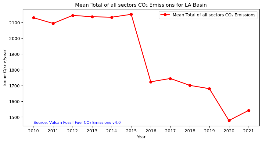
Summary
In this notebook, we have successfully completed the following steps for the Vulcan Fossil Fuel CO₂ Emissions dataset:
- Install and import the necessary libraries
- Fetch the collection from STAC using the appropriate endpoints
- Count the number of existing granules within the collection
- Map and compare the total fossil fuel CO₂ emissions for two distinctive months/years
- Generate zonal statistics for the area of interest (AOI)
- Plot a time series of mean total CO₂ emissions from all sectors for a specified region
If you have any questions regarding this user notebook, please contact us using the feedback form.