# Import the following libraries
# For fetching from the Raster API
import requests
# For making maps
import folium
import folium.plugins
from folium import Map, TileLayer
# For talking to the STAC API
from pystac_client import Client
# For working with data
import pandas as pd
# For making time series
import matplotlib.pyplot as plt
# For formatting date/time data
import datetime
# Custom functions for working with GHGC data via the API
import ghgc_utilsOCO-2 MIP Top-down CO₂ Budgets
Global, 1 degree resolution pilot top-down budgets of carbon dioxide emissions at 5 year intervals and national scales, version 1.
Author
Siddharth Chaudhary, Vishal Gaur
Published
August 1, 2023
Access this Notebook
You can launch this notebook in the US GHG Center JupyterHub (requires access) by clicking the following link: OCO-2 MIP Top-down CO₂ Budgets. If you are a new user, you should first sign up for the hub by filling out this request form and providing the required information.
If you do not have a US GHG Center Jupyterhub account, you can access this notebook through MyBinder by clicking the button below.
![]()
Table of Contents
Data Summary and Application
- Spatial coverage: Global
- Spatial resolution: 1° x 1°
- Temporal extent: 2015 – 2020
- Temporal resolution: Annual
- Unit: Grams of carbon dioxide per square meter per year (g CO₂/m²/yr)
- Utility: Climate Research
For more information, visit the OCO-2 MIP Top-down CO₂ Budgets data overview page.
About the Data
OCO-2 MIP Top-down CO₂ Budgets
The Committee on Earth Observation Satellites (CEOS) Atmospheric Composition - Virtual Constellation (AC-VC) Greenhouse Gas (GHG) team has generated the CEOS CO₂ Budgets dataset, which provides annual top-down carbon dioxide (CO₂) emissions and removals from 2015 - 2020 gridded globally at 1° resolution, and as national totals. Data is provided in units of grams of carbon dioxide per square meter per year (g CO₂/m2/yr). Only a subset of the full dataset is displayed in the US GHG Center explore view.
For more information regarding this dataset, please visit the OCO-2 MIP Top-down CO₂ Budgets data overview page.
Approach
- Identify available dates and temporal frequency of observations for the given collection using the US GHG Center (GHGC) Application Programming Interface (API)
/stacendpoint. The collection processed in this notebook is the OCO-2 MIP Top-down CO₂ Budgets data product. - Pass the STAC item into the raster API
/collections/{collection_id}/items/{item_id}/{tile_matrix_set_id}/tilejson.jsonendpoint. - Using
folium.plugins.DualMap, visualize two tiles (side-by-side), allowing time point comparison. - After the visualization, perform zonal statistics for a given polygon.
Terminology
Navigating data via the GHGC API, you will encounter terminology that is different from browsing in a typical filesystem. We’ll define some terms here which are used throughout this notebook.
catalog: All datasets available at the/stacendpointcollection: A specific dataset, e.g. OCO-2 MIP Top-down CO2 Budgetsitem: One data file (i.e. granule) in the dataset, e.g. one year of CO2 fluxesasset: A variable available within the granule, e.g. CO2 fluxes from crops, wood, or riversSTAC API: SpatioTemporal Asset Catalogs - Endpoint for fetching metadata about available datasetsRaster API: Endpoint for fetching data itself, for imagery and statistics
Install the Required Libraries
Required libraries are pre-installed on the US GHG Center Hub. If you need to run this notebook elsewhere, please install them with this line in a code cell:
%pip install requests folium rasterstats pystac_client pandas matplotlib –quiet
Query the STAC API
STAC API Collection Names
Now, you must fetch the dataset from the STAC API by defining its associated STAC API collection ID as a variable. The collection ID, also known as the collection name, for the OCO-2 MIP Top-down CO2 Budgets dataset is oco2-mip-co2budget-yeargrid-v1.
# Provide the STAC and RASTER API endpoints
# The endpoint is referring to a location within the API that executes a request on a data collection nesting on the server.

# The STAC API is a catalog of all the existing data collections that are stored in the GHG Center.
STAC_API_URL = "https://earth.gov/ghgcenter/api/stac"

# The RASTER API is used to fetch collections for visualization
RASTER_API_URL = "https://earth.gov/ghgcenter/api/raster"

# Define the collection name, used to fetch the dataset from the STAC API
collection_name = "oco2-mip-co2budget-yeargrid-v1"
<CollectionClient id=oco2-mip-co2budget-yeargrid-v1>
- type "Collection"
- id "oco2-mip-co2budget-yeargrid-v1"
- stac_version "1.1.0"
- description "This dataset contains top-down annual net land-atmosphere fluxes of CO₂ on a 1-degree grid for a six-year period (2015-2020) from an ensamble of atmospheric CO₂ inversions, as well as annual bottom-up estimates of fossil fuel emissions and lateral carbon fluxes due to crop trade, wood trade, river export and cement production. Annual changes (loss) in terrestrial carbon stocks are obtained by combining top-down and bottom-up estimates. The standard deviation for each variable is provided (std). IS layers assimilates in situ CO₂ mole fraction measurements from an international observational network. LNLG layers assimilates CO₂ measurements from the ACOS v10 algorithm which uses land nadir and land glint total column dry-air mole fractions observed by the OCO-2 satellite. LNLGIS layers assimilates both in situ and ACOS v10 OCO-2 land nadir and glint retrievals together. OG layers assimilates CO₂ measurements from the ACOS v10 algorithm using OCO-2 ocean glint retrievals. LNLGOGIS assimilates all sources together (in situ (IS), OCO-2 ACOS v10 land nadir and land glint (LNLG), OCO-2 ACOS v10 ocean glint (OG)). Data is provided in units of grams of carbon dioxide per square meter per year (g CO₂/m2/yr). The source dataset is titled Pilot top-down CO₂ budget constrained by the v10 OCO-2 MIP Version 1 and can be found at https://doi.org/10.48588/npf6-sw92"
links[] 5 items
0
- rel "items"
- href "https://earth.gov/ghgcenter/api/stac/collections/oco2-mip-co2budget-yeargrid-v1/items"
- type "application/geo+json"
1
- rel "parent"
- href "https://earth.gov/ghgcenter/api/stac/"
- type "application/json"
2
- rel "root"
- href "https://earth.gov/ghgcenter/api/stac"
- type "application/json"
- title "US GHG Center STAC API"
3
- rel "self"
- href "https://earth.gov/ghgcenter/api/stac/collections/oco2-mip-co2budget-yeargrid-v1"
- type "application/json"
4
- rel "http://www.opengis.net/def/rel/ogc/1.0/queryables"
- href "https://earth.gov/ghgcenter/api/stac/collections/oco2-mip-co2budget-yeargrid-v1/queryables"
- type "application/schema+json"
- title "Queryables"
stac_extensions[] 2 items
- 0 "https://stac-extensions.github.io/render/v1.0.0/schema.json"
- 1 "https://stac-extensions.github.io/item-assets/v1.0.0/schema.json"
renders
ff
assets[] 1 items
- 0 "ff"
- nodata 0
rescale[] 1 items
0[] 2 items
- 0 0
- 1 450
- colormap_name "purd"
crop
assets[] 1 items
- 0 "crop"
- nodata 0
rescale[] 1 items
0[] 2 items
- 0 -100
- 1 100
- colormap_name "coolwarm"
wood
assets[] 1 items
- 0 "wood"
- nodata 0
rescale[] 1 items
0[] 2 items
- 0 -100
- 1 100
- colormap_name "coolwarm"
river
assets[] 1 items
- 0 "river"
- nodata 0
rescale[] 1 items
0[] 2 items
- 0 -50
- 1 50
- colormap_name "coolwarm"
ff-std
assets[] 1 items
- 0 "ff-std"
- nodata 0
rescale[] 1 items
0[] 2 items
- 0 0
- 1 100
- colormap_name "purd"
crop-std
assets[] 1 items
- 0 "crop-std"
- nodata 0
rescale[] 1 items
0[] 2 items
- 0 0
- 1 50
- colormap_name "purd"
wood-std
assets[] 1 items
- 0 "wood-std"
- nodata 0
rescale[] 1 items
0[] 2 items
- 0 0
- 1 50
- colormap_name "purd"
dashboard
assets[] 1 items
- 0 "lnlgis-nbe"
- nodata 0
rescale[] 1 items
0[] 2 items
- 0 -1200
- 1 1200
- colormap_name "coolwarm"
river-std
assets[] 1 items
- 0 "river-std"
- nodata 0
rescale[] 1 items
0[] 2 items
- 0 0
- 1 60
- colormap_name "purd"
lnlgis-nbe
assets[] 1 items
- 0 "lnlgis-nbe"
- nodata 0
rescale[] 1 items
0[] 2 items
- 0 -1200
- 1 1200
- colormap_name "coolwarm"
lnlgis-nce
assets[] 1 items
- 0 "lnlgis-nce"
- nodata 0
rescale[] 1 items
0[] 2 items
- 0 -1200
- 1 1200
- colormap_name "coolwarm"
lnlgis-dc-loss
assets[] 1 items
- 0 "lnlgis-dc-loss"
- nodata 0
rescale[] 1 items
0[] 2 items
- 0 -600
- 1 600
- colormap_name "coolwarm"
lnlgis-nbe-std
assets[] 1 items
- 0 "lnlgis-nbe-std"
- nodata 0
rescale[] 1 items
0[] 2 items
- 0 0
- 1 1000
- colormap_name "purd"
lnlgis-nce-std
assets[] 1 items
- 0 "lnlgis-nce-std"
- nodata 0
rescale[] 1 items
0[] 2 items
- 0 0
- 1 1200
- colormap_name "purd"
lnlgis-dc-loss-std
assets[] 1 items
- 0 "lnlgis-dc-loss-std"
- nodata 0
rescale[] 1 items
0[] 2 items
- 0 0
- 1 800
- colormap_name "purd"
item_assets
ff
- type "image/tiff; application=geotiff; profile=cloud-optimized"
roles[] 2 items
- 0 "data"
- 1 "layer"
- title "Fossil Fuel and Cement Emissions"
- description "The burning of fossil fuels and release of carbon due to cement production, representing a flux of carbon from the land surface (geologic reservoir) to the atmosphere."
crop
- type "image/tiff; application=geotiff; profile=cloud-optimized"
roles[] 2 items
- 0 "data"
- 1 "layer"
- title "Lateral Crop Flux"
- description "The lateral flux of carbon in (positive) or out (negative) of a region due to agriculture."
wood
- type "image/tiff; application=geotiff; profile=cloud-optimized"
roles[] 2 items
- 0 "data"
- 1 "layer"
- title "Lateral Wood Flux"
- description "The lateral flux of carbon in (positive) or out (negative) of a region due to wood product harvesting and usage."
river
- type "image/tiff; application=geotiff; profile=cloud-optimized"
roles[] 2 items
- 0 "data"
- 1 "layer"
- title "Lateral River Flux"
- description "The lateral flux of carbon in (positive) or out (negative) of a region transported by the water cycle."
ff-std
- type "image/tiff; application=geotiff; profile=cloud-optimized"
roles[] 2 items
- 0 "data"
- 1 "layer"
- title "Fossil Fuel and Cement Emissions std"
- description "The burning of fossil fuels and release of carbon due to cement production, representing a flux of carbon from the land surface (geologic reservoir) to the atmosphere."
is-nbe
- type "image/tiff; application=geotiff; profile=cloud-optimized"
roles[] 2 items
- 0 "data"
- 1 "layer"
- title "In Situ Net Biosphere Exchange"
- description "Net flux of carbon from the terrestrial biosphere to the atmosphere due to biomass burning (BB) and Reco minus gross primary production (GPP). It includes both anthropogenic processes (e.g., deforestation, reforestation, farming) and natural processes (e.g., climate-variability-induced carbon fluxes, disturbances, recovery from disturbances)."
is-nce
- type "image/tiff; application=geotiff; profile=cloud-optimized"
roles[] 2 items
- 0 "data"
- 1 "layer"
- title "In Situ Terrestrial Net Carbon Exchange"
- description "Net flux of carbon from the surface to the atmosphere. For land, NCE can be defined as sum of NBE and fossil fuel and cement emissions."
crop-std
- type "image/tiff; application=geotiff; profile=cloud-optimized"
roles[] 2 items
- 0 "data"
- 1 "layer"
- title "Lateral Crop Flux std"
- description "The lateral flux of carbon in (positive) or out (negative) of a region due to agriculture."
lnlg-nbe
- type "image/tiff; application=geotiff; profile=cloud-optimized"
roles[] 2 items
- 0 "data"
- 1 "layer"
- title "Land Nadir and Land Glint Net Biosphere Exchange"
- description "Net flux of carbon from the terrestrial biosphere to the atmosphere due to biomass burning (BB) and Reco minus gross primary production (GPP). It includes both anthropogenic processes (e.g., deforestation, reforestation, farming) and natural processes (e.g., climate-variability-induced carbon fluxes, disturbances, recovery from disturbances."
lnlg-nce
- type "image/tiff; application=geotiff; profile=cloud-optimized"
roles[] 2 items
- 0 "data"
- 1 "layer"
- title "Land Nadir and Land Glint Terrestrial Net Carbon Exchange"
- description "Net flux of carbon from the surface to the atmosphere. For land, NCE can be defined as sum of NBE and fossil fuel and cement emissions."
wood-std
- type "image/tiff; application=geotiff; profile=cloud-optimized"
roles[] 2 items
- 0 "data"
- 1 "layer"
- title "Lateral Wood Flux std"
- description "The lateral flux of carbon in (positive) or out (negative) of a region due to wood product harvesting and usage."
river-std
- type "image/tiff; application=geotiff; profile=cloud-optimized"
roles[] 2 items
- 0 "data"
- 1 "layer"
- title "Lateral River Flux std"
- description "The lateral flux of carbon in (positive) or out (negative) of a region transported by the water cycle."
is-dc-loss
- type "image/tiff; application=geotiff; profile=cloud-optimized"
roles[] 2 items
- 0 "data"
- 1 "layer"
- title "In Situ Net Terrestrial Carbon Stock Loss"
- description "Positive values indicate a loss (decrease) of terrestrial carbon stocks (organic matter stored on land), including above- and below-ground biomass in ecosystems and biomass contained in anthropogenic products (lumber, cattle, etc.)."
is-nbe-std
- type "image/tiff; application=geotiff; profile=cloud-optimized"
roles[] 2 items
- 0 "data"
- 1 "layer"
- title "In Situ Net Biosphere Exchange std"
- description "Net flux of carbon from the terrestrial biosphere to the atmosphere due to biomass burning (BB) and Reco minus gross primary production (GPP). It includes both anthropogenic processes (e.g., deforestation, reforestation, farming) and natural processes (e.g., climate-variability-induced carbon fluxes, disturbances, recovery from disturbances."
is-nce-std
- type "image/tiff; application=geotiff; profile=cloud-optimized"
roles[] 2 items
- 0 "data"
- 1 "layer"
- title "In Situ Terrestrial Net Carbon Exchange std"
- description "Net flux of carbon from the surface to the atmosphere. For land, NCE can be defined as sum of NBE and fossil fuel and cement emissions."
lnlgis-nbe
- type "image/tiff; application=geotiff; profile=cloud-optimized"
roles[] 2 items
- 0 "data"
- 1 "layer"
- title "Land Nadir, Land Glint and In Situ Net Biosphere Exchange"
- description "Net flux of carbon from the terrestrial biosphere to the atmosphere due to biomass burning (BB) and Reco minus gross primary production (GPP). It includes both anthropogenic processes (e.g., deforestation, reforestation, farming) and natural processes (e.g., climate-variability-induced carbon fluxes, disturbances, recovery from disturbances."
lnlgis-nce
- type "image/tiff; application=geotiff; profile=cloud-optimized"
roles[] 2 items
- 0 "data"
- 1 "layer"
- title "Land Nadir, Land Glint and In Situ Terrestrial Net Carbon Exchange"
- description "Net flux of carbon from the surface to the atmosphere. For land, NCE can be defined as sum of NBE and fossil fuel and cement emissions."
lnlg-dc-loss
- type "image/tiff; application=geotiff; profile=cloud-optimized"
roles[] 2 items
- 0 "data"
- 1 "layer"
- title "Land Nadir and Land Glint Net Terrestrial Carbon Stock Loss"
- description "Positive values indicate a loss (decrease) of terrestrial carbon stocks (organic matter stored on land), including above- and below-ground biomass in ecosystems and biomass contained in anthropogenic products (lumber, cattle, etc.)."
lnlg-nbe-std
- type "image/tiff; application=geotiff; profile=cloud-optimized"
roles[] 2 items
- 0 "data"
- 1 "layer"
- title "Land Nadir and Land Glint Net Biosphere Exchange std"
- description "Net flux of carbon from the terrestrial biosphere to the atmosphere due to biomass burning (BB) and Reco minus gross primary production (GPP). It includes both anthropogenic processes (e.g., deforestation, reforestation, farming) and natural processes (e.g., climate-variability-induced carbon fluxes, disturbances, recovery from disturbances."
lnlg-nce-std
- type "image/tiff; application=geotiff; profile=cloud-optimized"
roles[] 2 items
- 0 "data"
- 1 "layer"
- title "Land Nadir and Land Glint Terrestrial Net Carbon Exchange std"
- description "Net flux of carbon from the surface to the atmosphere. For land, NCE can be defined as sum of NBE and fossil fuel and cement emissions."
lnlgogis-nbe
- type "image/tiff; application=geotiff; profile=cloud-optimized"
roles[] 2 items
- 0 "data"
- 1 "layer"
- title "Land Nadir, Land Glint, Ocean Glint and In Situ Net Biosphere Exchange"
- description "Net flux of carbon from the terrestrial biosphere to the atmosphere due to biomass burning (BB) and Reco minus gross primary production (GPP). It includes both anthropogenic processes (e.g., deforestation, reforestation, farming) and natural processes (e.g., climate-variability-induced carbon fluxes, disturbances, recovery from disturbances."
lnlgogis-nce
- type "image/tiff; application=geotiff; profile=cloud-optimized"
roles[] 2 items
- 0 "data"
- 1 "layer"
- title "Land Nadir, Land Glint, Ocean Glint and In Situ Terrestrial Net Carbon Exchange"
- description "Net flux of carbon from the surface to the atmosphere. For land, NCE can be defined as sum of NBE and fossil fuel and cement emissions."
is-dc-loss-std
- type "image/tiff; application=geotiff; profile=cloud-optimized"
roles[] 2 items
- 0 "data"
- 1 "layer"
- title "In Situ Net Terrestrial Carbon Stock Loss std"
- description "Positive values indicate a loss (decrease) of terrestrial carbon stocks (organic matter stored on land), including above- and below-ground biomass in ecosystems and biomass contained in anthropogenic products (lumber, cattle, etc.)."
lnlgis-dc-loss
- type "image/tiff; application=geotiff; profile=cloud-optimized"
roles[] 2 items
- 0 "data"
- 1 "layer"
- title "Land Nadir, Land Glint and In Situ Net Terrestrial Carbon Stock Loss"
- description "Positive values indicate a loss (decrease) of terrestrial carbon stocks (organic matter stored on land), including above- and below-ground biomass in ecosystems and biomass contained in anthropogenic products (lumber, cattle, etc.)."
lnlgis-nbe-std
- type "image/tiff; application=geotiff; profile=cloud-optimized"
roles[] 2 items
- 0 "data"
- 1 "layer"
- title "Land Nadir, Land Glint and In Situ Net Biosphere Exchange std"
- description "Net flux of carbon from the terrestrial biosphere to the atmosphere due to biomass burning (BB) and Reco minus gross primary production (GPP). It includes both anthropogenic processes (e.g., deforestation, reforestation, farming) and natural processes (e.g., climate-variability-induced carbon fluxes, disturbances, recovery from disturbances."
lnlgis-nce-std
- type "image/tiff; application=geotiff; profile=cloud-optimized"
roles[] 2 items
- 0 "data"
- 1 "layer"
- title "Land Nadir, Land Glint and In Situ Terrestrial Net Carbon Exchange std"
- description "Net flux of carbon from the surface to the atmosphere. For land, NCE can be defined as sum of NBE and fossil fuel and cement emissions."
lnlg-dc-loss-std
- type "image/tiff; application=geotiff; profile=cloud-optimized"
roles[] 2 items
- 0 "data"
- 1 "layer"
- title "Land Nadir and Land Glint Net Terrestrial Carbon Stock Loss std"
- description "Positive values indicate a loss (decrease) of terrestrial carbon stocks (organic matter stored on land), including above- and below-ground biomass in ecosystems and biomass contained in anthropogenic products (lumber, cattle, etc.)."
lnlgogis-dc-loss
- type "image/tiff; application=geotiff; profile=cloud-optimized"
roles[] 2 items
- 0 "data"
- 1 "layer"
- title "Land Nadir, Land Glint, Ocean Glint and In Situ Net Terrestrial Carbon Stock Loss"
- description "Positive values indicate a loss (decrease) of terrestrial carbon stocks (organic matter stored on land), including above- and below-ground biomass in ecosystems and biomass contained in anthropogenic products (lumber, cattle, etc.)."
lnlgogis-nbe-std
- type "image/tiff; application=geotiff; profile=cloud-optimized"
roles[] 2 items
- 0 "data"
- 1 "layer"
- title "Land Nadir, Land Glint, Ocean Glint and In Situ Net Biosphere Exchange"
- description "Net flux of carbon from the terrestrial biosphere to the atmosphere due to biomass burning (BB) and Reco minus gross primary production (GPP). It includes both anthropogenic processes (e.g., deforestation, reforestation, farming) and natural processes (e.g., climate-variability-induced carbon fluxes, disturbances, recovery from disturbances."
lnlgogis-nce-std
- type "image/tiff; application=geotiff; profile=cloud-optimized"
roles[] 2 items
- 0 "data"
- 1 "layer"
- title "Land Nadir, Land Glint, Ocean Glint and In Situ Terrestrial Net Carbon Exchange std"
- description "Net flux of carbon from the surface to the atmosphere. For land, NCE can be defined as sum of NBE and fossil fuel and cement emissions."
lnlgis-dc-loss-std
- type "image/tiff; application=geotiff; profile=cloud-optimized"
roles[] 2 items
- 0 "data"
- 1 "layer"
- title "Land Nadir, Land Glint and In Situ Net Terrestrial Carbon Stock Loss std"
- description "Positive values indicate a loss (decrease) of terrestrial carbon stocks (organic matter stored on land), including above- and below-ground biomass in ecosystems and biomass contained in anthropogenic products (lumber, cattle, etc.)."
lnlgogis-dc-loss-std
- type "image/tiff; application=geotiff; profile=cloud-optimized"
roles[] 2 items
- 0 "data"
- 1 "layer"
- title "Land Nadir, Land Glint, Ocean Glint and In Situ Net Terrestrial Carbon Stock Loss std"
- description "Positive values indicate a loss (decrease) of terrestrial carbon stocks (organic matter stored on land), including above- and below-ground biomass in ecosystems and biomass contained in anthropogenic products (lumber, cattle, etc.)."
- dashboard:is_periodic True
- dashboard:time_density "year"
- title "OCO-2 MIP Top-down CO₂ Budgets v1"
extent
spatial
bbox[] 1 items
0[] 4 items
- 0 -180.0
- 1 -90.0
- 2 180.0
- 3 90.0
temporal
interval[] 1 items
0[] 2 items
- 0 "2015-01-01T00:00:00Z"
- 1 "2020-01-01T00:00:00Z"
- license "CC-BY-4.0"
summaries
datetime[] 2 items
- 0 "2015-01-01T00:00:00+00:00"
- 1 "2020-01-01T00:00:00+00:00"
Examining the contents of our collection under the temporal variable, we see that the data is available from January 2015 to January 2020. By looking at the dashboard:time density, we observe that the periodic frequency of these observations is yearly.
Found 6 items
<Item id=oco2-mip-co2budget-yeargrid-v1-2020>
- type "Feature"
- stac_version "1.1.0"
stac_extensions[] 0 items
- id "oco2-mip-co2budget-yeargrid-v1-2020"
geometry
- type "Polygon"
coordinates[] 1 items
0[] 5 items
0[] 2 items
- 0 -180
- 1 -90
1[] 2 items
- 0 180
- 1 -90
2[] 2 items
- 0 180
- 1 90
3[] 2 items
- 0 -180
- 1 90
4[] 2 items
- 0 -180
- 1 -90
bbox[] 4 items
- 0 -180.0
- 1 -90.0
- 2 180.0
- 3 90.0
properties
- end_datetime "2020-12-31T00:00:00+00:00"
- start_datetime "2020-01-01T00:00:00+00:00"
- datetime None
links[] 5 items
0
- rel "collection"
- href "https://earth.gov/ghgcenter/api/stac/collections/oco2-mip-co2budget-yeargrid-v1"
- type "application/json"
1
- rel "parent"
- href "https://earth.gov/ghgcenter/api/stac/collections/oco2-mip-co2budget-yeargrid-v1"
- type "application/json"
2
- rel "root"
- href "https://earth.gov/ghgcenter/api/stac"
- type "application/json"
- title "US GHG Center STAC API"
3
- rel "self"
- href "https://earth.gov/ghgcenter/api/stac/collections/oco2-mip-co2budget-yeargrid-v1/items/oco2-mip-co2budget-yeargrid-v1-2020"
- type "application/geo+json"
4
- rel "preview"
- href "https://earth.gov/ghgcenter/api/raster/collections/oco2-mip-co2budget-yeargrid-v1/items/oco2-mip-co2budget-yeargrid-v1-2020/WebMercatorQuad/map?assets=lnlgis-nbe&nodata=0&rescale=-1200%2C1200&colormap_name=coolwarm"
- type "text/html"
- title "Map of Item"
assets
ff
- href "s3://ghgc-data-store/oco2-mip-co2budget-yeargrid-v1/pilot_topdown_FF_CO2_Budget_grid_v1_2020.tif"
- type "image/tiff; application=geotiff; profile=cloud-optimized"
- title "Fossil Fuel and Cement Emissions"
- description "The burning of fossil fuels and release of carbon due to cement production, representing a flux of carbon from the land surface (geologic reservoir) to the atmosphere."
proj:bbox[] 4 items
- 0 -180.0
- 1 -90.0
- 2 180.0
- 3 90.0
- proj:epsg 4326.0
proj:shape[] 2 items
- 0 180.0
- 1 360.0
raster:bands[] 1 items
0
- scale 1.0
- offset 0.0
- sampling "area"
- data_type "float64"
histogram
- max 25762.3125
- min 0.0
- count 11.0
buckets[] 10 items
- 0 64516.0
- 1 199.0
- 2 48.0
- 3 17.0
- 4 10.0
- 5 4.0
- 6 1.0
- 7 0.0
- 8 3.0
- 9 2.0
statistics
- mean 54.68926524648964
- stddev 442.23989014106485
- maximum 25762.3125
- minimum 0.0
- valid_percent 0.00154320987654321
proj:geometry
- type "Polygon"
coordinates[] 1 items
0[] 5 items
0[] 2 items
- 0 -180.0
- 1 -90.0
1[] 2 items
- 0 180.0
- 1 -90.0
2[] 2 items
- 0 180.0
- 1 90.0
3[] 2 items
- 0 -180.0
- 1 90.0
4[] 2 items
- 0 -180.0
- 1 -90.0
proj:projjson
id
- code 4326.0
- authority "EPSG"
- name "WGS 84"
- type "GeographicCRS"
datum
- name "World Geodetic System 1984"
- type "GeodeticReferenceFrame"
ellipsoid
- name "WGS 84"
- semi_major_axis 6378137.0
- inverse_flattening 298.257223563
- $schema "https://proj.org/schemas/v0.4/projjson.schema.json"
coordinate_system
axis[] 2 items
0
- name "Geodetic latitude"
- unit "degree"
- direction "north"
- abbreviation "Lat"
1
- name "Geodetic longitude"
- unit "degree"
- direction "east"
- abbreviation "Lon"
- subtype "ellipsoidal"
proj:transform[] 9 items
- 0 1.0
- 1 0.0
- 2 -180.0
- 3 0.0
- 4 -1.0
- 5 90.0
- 6 0.0
- 7 0.0
- 8 1.0
roles[] 2 items
- 0 "data"
- 1 "layer"
crop
- href "s3://ghgc-data-store/oco2-mip-co2budget-yeargrid-v1/pilot_topdown_Crop_CO2_Budget_grid_v1_2020.tif"
- type "image/tiff; application=geotiff; profile=cloud-optimized"
- title "Lateral Crop Flux"
- description "The lateral flux of carbon in (positive) or out (negative) of a region due to agriculture."
proj:bbox[] 4 items
- 0 -180.0
- 1 -90.0
- 2 180.0
- 3 90.0
- proj:epsg 4326.0
proj:shape[] 2 items
- 0 180.0
- 1 360.0
raster:bands[] 1 items
0
- scale 1.0
- offset 0.0
- sampling "area"
- data_type "float64"
histogram
- max 1413.4342939282176
- min -821.2316120182234
- count 11.0
buckets[] 10 items
- 0 1.0
- 1 7.0
- 2 71.0
- 3 64473.0
- 4 222.0
- 5 17.0
- 6 5.0
- 7 2.0
- 8 0.0
- 9 2.0
statistics
- mean -0.0848818515530641
- stddev 19.816472674277588
- maximum 1413.4342939282176
- minimum -821.2316120182234
- valid_percent 0.00154320987654321
proj:geometry
- type "Polygon"
coordinates[] 1 items
0[] 5 items
0[] 2 items
- 0 -180.0
- 1 -90.0
1[] 2 items
- 0 180.0
- 1 -90.0
2[] 2 items
- 0 180.0
- 1 90.0
3[] 2 items
- 0 -180.0
- 1 90.0
4[] 2 items
- 0 -180.0
- 1 -90.0
proj:projjson
id
- code 4326.0
- authority "EPSG"
- name "WGS 84"
- type "GeographicCRS"
datum
- name "World Geodetic System 1984"
- type "GeodeticReferenceFrame"
ellipsoid
- name "WGS 84"
- semi_major_axis 6378137.0
- inverse_flattening 298.257223563
- $schema "https://proj.org/schemas/v0.4/projjson.schema.json"
coordinate_system
axis[] 2 items
0
- name "Geodetic latitude"
- unit "degree"
- direction "north"
- abbreviation "Lat"
1
- name "Geodetic longitude"
- unit "degree"
- direction "east"
- abbreviation "Lon"
- subtype "ellipsoidal"
proj:transform[] 9 items
- 0 1.0
- 1 0.0
- 2 -180.0
- 3 0.0
- 4 -1.0
- 5 90.0
- 6 0.0
- 7 0.0
- 8 1.0
roles[] 2 items
- 0 "data"
- 1 "layer"
wood
- href "s3://ghgc-data-store/oco2-mip-co2budget-yeargrid-v1/pilot_topdown_Wood_CO2_Budget_grid_v1_2020.tif"
- type "image/tiff; application=geotiff; profile=cloud-optimized"
- title "Lateral Wood Flux"
- description "The lateral flux of carbon in (positive) or out (negative) of a region due to wood product harvesting and usage."
proj:bbox[] 4 items
- 0 -180.0
- 1 -90.0
- 2 180.0
- 3 90.0
- proj:epsg 4326.0
proj:shape[] 2 items
- 0 180.0
- 1 360.0
raster:bands[] 1 items
0
- scale 1.0
- offset 0.0
- sampling "area"
- data_type "float64"
histogram
- max 886.8267457880838
- min -893.4090768667005
- count 11.0
buckets[] 10 items
- 0 1.0
- 1 0.0
- 2 2.0
- 3 54.0
- 4 4763.0
- 5 59968.0
- 6 10.0
- 7 1.0
- 8 0.0
- 9 1.0
statistics
- mean -1.6227997301943906
- stddev 14.426756498712097
- maximum 886.8267457880838
- minimum -893.4090768667005
- valid_percent 0.00154320987654321
proj:geometry
- type "Polygon"
coordinates[] 1 items
0[] 5 items
0[] 2 items
- 0 -180.0
- 1 -90.0
1[] 2 items
- 0 180.0
- 1 -90.0
2[] 2 items
- 0 180.0
- 1 90.0
3[] 2 items
- 0 -180.0
- 1 90.0
4[] 2 items
- 0 -180.0
- 1 -90.0
proj:projjson
id
- code 4326.0
- authority "EPSG"
- name "WGS 84"
- type "GeographicCRS"
datum
- name "World Geodetic System 1984"
- type "GeodeticReferenceFrame"
ellipsoid
- name "WGS 84"
- semi_major_axis 6378137.0
- inverse_flattening 298.257223563
- $schema "https://proj.org/schemas/v0.4/projjson.schema.json"
coordinate_system
axis[] 2 items
0
- name "Geodetic latitude"
- unit "degree"
- direction "north"
- abbreviation "Lat"
1
- name "Geodetic longitude"
- unit "degree"
- direction "east"
- abbreviation "Lon"
- subtype "ellipsoidal"
proj:transform[] 9 items
- 0 1.0
- 1 0.0
- 2 -180.0
- 3 0.0
- 4 -1.0
- 5 90.0
- 6 0.0
- 7 0.0
- 8 1.0
roles[] 2 items
- 0 "data"
- 1 "layer"
river
- href "s3://ghgc-data-store/oco2-mip-co2budget-yeargrid-v1/pilot_topdown_River_CO2_Budget_grid_v1_2020.tif"
- type "image/tiff; application=geotiff; profile=cloud-optimized"
- title "Lateral River Flux"
- description "The lateral flux of carbon in (positive) or out (negative) of a region transported by the water cycle."
proj:bbox[] 4 items
- 0 -180.0
- 1 -90.0
- 2 180.0
- 3 90.0
- proj:epsg 4326.0
proj:shape[] 2 items
- 0 180.0
- 1 360.0
raster:bands[] 1 items
0
- scale 1.0
- offset 0.0
- sampling "area"
- data_type "float64"
histogram
- max 230.29083544674185
- min -128.99315231552467
- count 11.0
buckets[] 10 items
- 0 4.0
- 1 25.0
- 2 547.0
- 3 63696.0
- 4 403.0
- 5 66.0
- 6 38.0
- 7 9.0
- 8 10.0
- 9 2.0
statistics
- mean -0.9365037131734213
- stddev 6.741980166906525
- maximum 230.29083544674185
- minimum -128.99315231552467
- valid_percent 0.00154320987654321
proj:geometry
- type "Polygon"
coordinates[] 1 items
0[] 5 items
0[] 2 items
- 0 -180.0
- 1 -90.0
1[] 2 items
- 0 180.0
- 1 -90.0
2[] 2 items
- 0 180.0
- 1 90.0
3[] 2 items
- 0 -180.0
- 1 90.0
4[] 2 items
- 0 -180.0
- 1 -90.0
proj:projjson
id
- code 4326.0
- authority "EPSG"
- name "WGS 84"
- type "GeographicCRS"
datum
- name "World Geodetic System 1984"
- type "GeodeticReferenceFrame"
ellipsoid
- name "WGS 84"
- semi_major_axis 6378137.0
- inverse_flattening 298.257223563
- $schema "https://proj.org/schemas/v0.4/projjson.schema.json"
coordinate_system
axis[] 2 items
0
- name "Geodetic latitude"
- unit "degree"
- direction "north"
- abbreviation "Lat"
1
- name "Geodetic longitude"
- unit "degree"
- direction "east"
- abbreviation "Lon"
- subtype "ellipsoidal"
proj:transform[] 9 items
- 0 1.0
- 1 0.0
- 2 -180.0
- 3 0.0
- 4 -1.0
- 5 90.0
- 6 0.0
- 7 0.0
- 8 1.0
roles[] 2 items
- 0 "data"
- 1 "layer"
ff-std
- href "s3://ghgc-data-store/oco2-mip-co2budget-yeargrid-v1/pilot_topdown_FF_std_CO2_Budget_grid_v1_2020.tif"
- type "image/tiff; application=geotiff; profile=cloud-optimized"
- title "Fossil Fuel and Cement Emissions std"
- description "The burning of fossil fuels and release of carbon due to cement production, representing a flux of carbon from the land surface (geologic reservoir) to the atmosphere."
proj:bbox[] 4 items
- 0 -180.0
- 1 -90.0
- 2 180.0
- 3 90.0
- proj:epsg 4326.0
proj:shape[] 2 items
- 0 180.0
- 1 360.0
raster:bands[] 1 items
0
- scale 1.0
- offset 0.0
- sampling "area"
- data_type "float64"
histogram
- max 23231.900390625
- min 0.0
- count 11.0
buckets[] 10 items
- 0 64705.0
- 1 76.0
- 2 11.0
- 3 3.0
- 4 1.0
- 5 1.0
- 6 2.0
- 7 0.0
- 8 0.0
- 9 1.0
statistics
- mean 26.378356791047626
- stddev 233.78396982573136
- maximum 23231.900390625
- minimum 0.0
- valid_percent 0.00154320987654321
proj:geometry
- type "Polygon"
coordinates[] 1 items
0[] 5 items
0[] 2 items
- 0 -180.0
- 1 -90.0
1[] 2 items
- 0 180.0
- 1 -90.0
2[] 2 items
- 0 180.0
- 1 90.0
3[] 2 items
- 0 -180.0
- 1 90.0
4[] 2 items
- 0 -180.0
- 1 -90.0
proj:projjson
id
- code 4326.0
- authority "EPSG"
- name "WGS 84"
- type "GeographicCRS"
datum
- name "World Geodetic System 1984"
- type "GeodeticReferenceFrame"
ellipsoid
- name "WGS 84"
- semi_major_axis 6378137.0
- inverse_flattening 298.257223563
- $schema "https://proj.org/schemas/v0.4/projjson.schema.json"
coordinate_system
axis[] 2 items
0
- name "Geodetic latitude"
- unit "degree"
- direction "north"
- abbreviation "Lat"
1
- name "Geodetic longitude"
- unit "degree"
- direction "east"
- abbreviation "Lon"
- subtype "ellipsoidal"
proj:transform[] 9 items
- 0 1.0
- 1 0.0
- 2 -180.0
- 3 0.0
- 4 -1.0
- 5 90.0
- 6 0.0
- 7 0.0
- 8 1.0
roles[] 2 items
- 0 "data"
- 1 "layer"
is-nbe
- href "s3://ghgc-data-store/oco2-mip-co2budget-yeargrid-v1/pilot_topdown_IS_NBE_CO2_Budget_grid_v1_2020.tif"
- type "image/tiff; application=geotiff; profile=cloud-optimized"
- title "In Situ Net Biosphere Exchange"
- description "Net flux of carbon from the terrestrial biosphere to the atmosphere due to biomass burning (BB) and Reco minus gross primary production (GPP). It includes both anthropogenic processes (e.g., deforestation, reforestation, farming) and natural processes (e.g., climate-variability-induced carbon fluxes, disturbances, recovery from disturbances)."
proj:bbox[] 4 items
- 0 -180.0
- 1 -90.0
- 2 180.0
- 3 90.0
- proj:epsg 4326.0
proj:shape[] 2 items
- 0 180.0
- 1 360.0
raster:bands[] 1 items
0
- scale 1.0
- offset 0.0
- sampling "area"
- data_type "float64"
histogram
- max 1149.6695556640625
- min -1408.24169921875
- count 11.0
buckets[] 10 items
- 0 16.0
- 1 35.0
- 2 108.0
- 3 616.0
- 4 3339.0
- 5 59909.0
- 6 676.0
- 7 88.0
- 8 12.0
- 9 1.0
statistics
- mean -17.434049799347616
- stddev 89.42319485219821
- maximum 1149.6695556640625
- minimum -1408.24169921875
- valid_percent 0.00154320987654321
proj:geometry
- type "Polygon"
coordinates[] 1 items
0[] 5 items
0[] 2 items
- 0 -180.0
- 1 -90.0
1[] 2 items
- 0 180.0
- 1 -90.0
2[] 2 items
- 0 180.0
- 1 90.0
3[] 2 items
- 0 -180.0
- 1 90.0
4[] 2 items
- 0 -180.0
- 1 -90.0
proj:projjson
id
- code 4326.0
- authority "EPSG"
- name "WGS 84"
- type "GeographicCRS"
datum
- name "World Geodetic System 1984"
- type "GeodeticReferenceFrame"
ellipsoid
- name "WGS 84"
- semi_major_axis 6378137.0
- inverse_flattening 298.257223563
- $schema "https://proj.org/schemas/v0.4/projjson.schema.json"
coordinate_system
axis[] 2 items
0
- name "Geodetic latitude"
- unit "degree"
- direction "north"
- abbreviation "Lat"
1
- name "Geodetic longitude"
- unit "degree"
- direction "east"
- abbreviation "Lon"
- subtype "ellipsoidal"
proj:transform[] 9 items
- 0 1.0
- 1 0.0
- 2 -180.0
- 3 0.0
- 4 -1.0
- 5 90.0
- 6 0.0
- 7 0.0
- 8 1.0
roles[] 2 items
- 0 "data"
- 1 "layer"
is-nce
- href "s3://ghgc-data-store/oco2-mip-co2budget-yeargrid-v1/pilot_topdown_IS_NCE_CO2_Budget_grid_v1_2020.tif"
- type "image/tiff; application=geotiff; profile=cloud-optimized"
- title "In Situ Terrestrial Net Carbon Exchange"
- description "Net flux of carbon from the surface to the atmosphere. For land, NCE can be defined as sum of NBE and fossil fuel and cement emissions."
proj:bbox[] 4 items
- 0 -180.0
- 1 -90.0
- 2 180.0
- 3 90.0
- proj:epsg 4326.0
proj:shape[] 2 items
- 0 180.0
- 1 360.0
raster:bands[] 1 items
0
- scale 1.0
- offset 0.0
- sampling "area"
- data_type "float64"
histogram
- max 25703.37777709961
- min -1226.5958404541016
- count 11.0
buckets[] 10 items
- 0 64278.0
- 1 400.0
- 2 72.0
- 3 26.0
- 4 13.0
- 5 4.0
- 6 2.0
- 7 0.0
- 8 3.0
- 9 2.0
statistics
- mean 37.255215447142035
- stddev 437.1998693275883
- maximum 25703.37777709961
- minimum -1226.5958404541016
- valid_percent 0.00154320987654321
proj:geometry
- type "Polygon"
coordinates[] 1 items
0[] 5 items
0[] 2 items
- 0 -180.0
- 1 -90.0
1[] 2 items
- 0 180.0
- 1 -90.0
2[] 2 items
- 0 180.0
- 1 90.0
3[] 2 items
- 0 -180.0
- 1 90.0
4[] 2 items
- 0 -180.0
- 1 -90.0
proj:projjson
id
- code 4326.0
- authority "EPSG"
- name "WGS 84"
- type "GeographicCRS"
datum
- name "World Geodetic System 1984"
- type "GeodeticReferenceFrame"
ellipsoid
- name "WGS 84"
- semi_major_axis 6378137.0
- inverse_flattening 298.257223563
- $schema "https://proj.org/schemas/v0.4/projjson.schema.json"
coordinate_system
axis[] 2 items
0
- name "Geodetic latitude"
- unit "degree"
- direction "north"
- abbreviation "Lat"
1
- name "Geodetic longitude"
- unit "degree"
- direction "east"
- abbreviation "Lon"
- subtype "ellipsoidal"
proj:transform[] 9 items
- 0 1.0
- 1 0.0
- 2 -180.0
- 3 0.0
- 4 -1.0
- 5 90.0
- 6 0.0
- 7 0.0
- 8 1.0
roles[] 2 items
- 0 "data"
- 1 "layer"
crop-std
- href "s3://ghgc-data-store/oco2-mip-co2budget-yeargrid-v1/pilot_topdown_Crop_std_CO2_Budget_grid_v1_2020.tif"
- type "image/tiff; application=geotiff; profile=cloud-optimized"
- title "Lateral Crop Flux std"
- description "The lateral flux of carbon in (positive) or out (negative) of a region due to agriculture."
proj:bbox[] 4 items
- 0 -180.0
- 1 -90.0
- 2 180.0
- 3 90.0
- proj:epsg 4326.0
proj:shape[] 2 items
- 0 180.0
- 1 360.0
raster:bands[] 1 items
0
- scale 1.0
- offset 0.0
- sampling "area"
- data_type "float64"
histogram
- max 424.0302881784653
- min 0.0
- count 11.0
buckets[] 10 items
- 0 64612.0
- 1 144.0
- 2 29.0
- 3 7.0
- 4 3.0
- 5 3.0
- 6 0.0
- 7 0.0
- 8 1.0
- 9 1.0
statistics
- mean 0.9286867985398175
- stddev 5.872011776754035
- maximum 424.0302881784653
- minimum 0.0
- valid_percent 0.00154320987654321
proj:geometry
- type "Polygon"
coordinates[] 1 items
0[] 5 items
0[] 2 items
- 0 -180.0
- 1 -90.0
1[] 2 items
- 0 180.0
- 1 -90.0
2[] 2 items
- 0 180.0
- 1 90.0
3[] 2 items
- 0 -180.0
- 1 90.0
4[] 2 items
- 0 -180.0
- 1 -90.0
proj:projjson
id
- code 4326.0
- authority "EPSG"
- name "WGS 84"
- type "GeographicCRS"
datum
- name "World Geodetic System 1984"
- type "GeodeticReferenceFrame"
ellipsoid
- name "WGS 84"
- semi_major_axis 6378137.0
- inverse_flattening 298.257223563
- $schema "https://proj.org/schemas/v0.4/projjson.schema.json"
coordinate_system
axis[] 2 items
0
- name "Geodetic latitude"
- unit "degree"
- direction "north"
- abbreviation "Lat"
1
- name "Geodetic longitude"
- unit "degree"
- direction "east"
- abbreviation "Lon"
- subtype "ellipsoidal"
proj:transform[] 9 items
- 0 1.0
- 1 0.0
- 2 -180.0
- 3 0.0
- 4 -1.0
- 5 90.0
- 6 0.0
- 7 0.0
- 8 1.0
roles[] 2 items
- 0 "data"
- 1 "layer"
lnlg-nbe
- href "s3://ghgc-data-store/oco2-mip-co2budget-yeargrid-v1/pilot_topdown_LNLG_NBE_CO2_Budget_grid_v1_2020.tif"
- type "image/tiff; application=geotiff; profile=cloud-optimized"
- title "Land Nadir and Land Glint Net Biosphere Exchange"
- description "Net flux of carbon from the terrestrial biosphere to the atmosphere due to biomass burning (BB) and Reco minus gross primary production (GPP). It includes both anthropogenic processes (e.g., deforestation, reforestation, farming) and natural processes (e.g., climate-variability-induced carbon fluxes, disturbances, recovery from disturbances."
proj:bbox[] 4 items
- 0 -180.0
- 1 -90.0
- 2 180.0
- 3 90.0
- proj:epsg 4326.0
proj:shape[] 2 items
- 0 180.0
- 1 360.0
raster:bands[] 1 items
0
- scale 1.0
- offset 0.0
- sampling "area"
- data_type "float64"
histogram
- max 2599.83935546875
- min -1888.9810791015625
- count 11.0
buckets[] 10 items
- 0 4.0
- 1 36.0
- 2 774.0
- 3 4318.0
- 4 58979.0
- 5 624.0
- 6 34.0
- 7 14.0
- 8 12.0
- 9 5.0
statistics
- mean -15.447162739865497
- stddev 132.6736652625944
- maximum 2599.83935546875
- minimum -1888.9810791015625
- valid_percent 0.00154320987654321
proj:geometry
- type "Polygon"
coordinates[] 1 items
0[] 5 items
0[] 2 items
- 0 -180.0
- 1 -90.0
1[] 2 items
- 0 180.0
- 1 -90.0
2[] 2 items
- 0 180.0
- 1 90.0
3[] 2 items
- 0 -180.0
- 1 90.0
4[] 2 items
- 0 -180.0
- 1 -90.0
proj:projjson
id
- code 4326.0
- authority "EPSG"
- name "WGS 84"
- type "GeographicCRS"
datum
- name "World Geodetic System 1984"
- type "GeodeticReferenceFrame"
ellipsoid
- name "WGS 84"
- semi_major_axis 6378137.0
- inverse_flattening 298.257223563
- $schema "https://proj.org/schemas/v0.4/projjson.schema.json"
coordinate_system
axis[] 2 items
0
- name "Geodetic latitude"
- unit "degree"
- direction "north"
- abbreviation "Lat"
1
- name "Geodetic longitude"
- unit "degree"
- direction "east"
- abbreviation "Lon"
- subtype "ellipsoidal"
proj:transform[] 9 items
- 0 1.0
- 1 0.0
- 2 -180.0
- 3 0.0
- 4 -1.0
- 5 90.0
- 6 0.0
- 7 0.0
- 8 1.0
roles[] 2 items
- 0 "data"
- 1 "layer"
lnlg-nce
- href "s3://ghgc-data-store/oco2-mip-co2budget-yeargrid-v1/pilot_topdown_LNLG_NCE_CO2_Budget_grid_v1_2020.tif"
- type "image/tiff; application=geotiff; profile=cloud-optimized"
- title "Land Nadir and Land Glint Terrestrial Net Carbon Exchange"
- description "Net flux of carbon from the surface to the atmosphere. For land, NCE can be defined as sum of NBE and fossil fuel and cement emissions."
proj:bbox[] 4 items
- 0 -180.0
- 1 -90.0
- 2 180.0
- 3 90.0
- proj:epsg 4326.0
proj:shape[] 2 items
- 0 180.0
- 1 360.0
raster:bands[] 1 items
0
- scale 1.0
- offset 0.0
- sampling "area"
- data_type "float64"
histogram
- max 25567.622344970703
- min -1853.1165390014648
- count 11.0
buckets[] 10 items
- 0 63941.0
- 1 720.0
- 2 81.0
- 3 33.0
- 4 14.0
- 5 4.0
- 6 2.0
- 7 0.0
- 8 3.0
- 9 2.0
statistics
- mean 39.24210250662415
- stddev 434.0339466646377
- maximum 25567.622344970703
- minimum -1853.1165390014648
- valid_percent 0.00154320987654321
proj:geometry
- type "Polygon"
coordinates[] 1 items
0[] 5 items
0[] 2 items
- 0 -180.0
- 1 -90.0
1[] 2 items
- 0 180.0
- 1 -90.0
2[] 2 items
- 0 180.0
- 1 90.0
3[] 2 items
- 0 -180.0
- 1 90.0
4[] 2 items
- 0 -180.0
- 1 -90.0
proj:projjson
id
- code 4326.0
- authority "EPSG"
- name "WGS 84"
- type "GeographicCRS"
datum
- name "World Geodetic System 1984"
- type "GeodeticReferenceFrame"
ellipsoid
- name "WGS 84"
- semi_major_axis 6378137.0
- inverse_flattening 298.257223563
- $schema "https://proj.org/schemas/v0.4/projjson.schema.json"
coordinate_system
axis[] 2 items
0
- name "Geodetic latitude"
- unit "degree"
- direction "north"
- abbreviation "Lat"
1
- name "Geodetic longitude"
- unit "degree"
- direction "east"
- abbreviation "Lon"
- subtype "ellipsoidal"
proj:transform[] 9 items
- 0 1.0
- 1 0.0
- 2 -180.0
- 3 0.0
- 4 -1.0
- 5 90.0
- 6 0.0
- 7 0.0
- 8 1.0
roles[] 2 items
- 0 "data"
- 1 "layer"
wood-std
- href "s3://ghgc-data-store/oco2-mip-co2budget-yeargrid-v1/pilot_topdown_Wood_std_CO2_Budget_grid_v1_2020.tif"
- type "image/tiff; application=geotiff; profile=cloud-optimized"
- title "Lateral Wood Flux std"
- description "The lateral flux of carbon in (positive) or out (negative) of a region due to wood product harvesting and usage."
proj:bbox[] 4 items
- 0 -180.0
- 1 -90.0
- 2 180.0
- 3 90.0
- proj:epsg 4326.0
proj:shape[] 2 items
- 0 180.0
- 1 360.0
raster:bands[] 1 items
0
- scale 1.0
- offset 0.0
- sampling "area"
- data_type "float64"
histogram
- max 268.02272306001015
- min 0.0
- count 11.0
buckets[] 10 items
- 0 64457.0
- 1 269.0
- 2 57.0
- 3 12.0
- 4 2.0
- 5 1.0
- 6 0.0
- 7 0.0
- 8 0.0
- 9 2.0
statistics
- mean 0.7520992161897981
- stddev 4.289892440653641
- maximum 268.02272306001015
- minimum 0.0
- valid_percent 0.00154320987654321
proj:geometry
- type "Polygon"
coordinates[] 1 items
0[] 5 items
0[] 2 items
- 0 -180.0
- 1 -90.0
1[] 2 items
- 0 180.0
- 1 -90.0
2[] 2 items
- 0 180.0
- 1 90.0
3[] 2 items
- 0 -180.0
- 1 90.0
4[] 2 items
- 0 -180.0
- 1 -90.0
proj:projjson
id
- code 4326.0
- authority "EPSG"
- name "WGS 84"
- type "GeographicCRS"
datum
- name "World Geodetic System 1984"
- type "GeodeticReferenceFrame"
ellipsoid
- name "WGS 84"
- semi_major_axis 6378137.0
- inverse_flattening 298.257223563
- $schema "https://proj.org/schemas/v0.4/projjson.schema.json"
coordinate_system
axis[] 2 items
0
- name "Geodetic latitude"
- unit "degree"
- direction "north"
- abbreviation "Lat"
1
- name "Geodetic longitude"
- unit "degree"
- direction "east"
- abbreviation "Lon"
- subtype "ellipsoidal"
proj:transform[] 9 items
- 0 1.0
- 1 0.0
- 2 -180.0
- 3 0.0
- 4 -1.0
- 5 90.0
- 6 0.0
- 7 0.0
- 8 1.0
roles[] 2 items
- 0 "data"
- 1 "layer"
river-std
- href "s3://ghgc-data-store/oco2-mip-co2budget-yeargrid-v1/pilot_topdown_River_std_CO2_Budget_grid_v1_2020.tif"
- type "image/tiff; application=geotiff; profile=cloud-optimized"
- title "Lateral River Flux std"
- description "The lateral flux of carbon in (positive) or out (negative) of a region transported by the water cycle."
proj:bbox[] 4 items
- 0 -180.0
- 1 -90.0
- 2 180.0
- 3 90.0
- proj:epsg 4326.0
proj:shape[] 2 items
- 0 180.0
- 1 360.0
raster:bands[] 1 items
0
- scale 1.0
- offset 0.0
- sampling "area"
- data_type "float64"
histogram
- max 138.1745012680451
- min 0.0
- count 11.0
buckets[] 10 items
- 0 64020.0
- 1 586.0
- 2 94.0
- 3 42.0
- 4 35.0
- 5 8.0
- 6 3.0
- 7 8.0
- 8 3.0
- 9 1.0
statistics
- mean 1.1315162852460954
- stddev 3.9241498156278833
- maximum 138.1745012680451
- minimum 0.0
- valid_percent 0.00154320987654321
proj:geometry
- type "Polygon"
coordinates[] 1 items
0[] 5 items
0[] 2 items
- 0 -180.0
- 1 -90.0
1[] 2 items
- 0 180.0
- 1 -90.0
2[] 2 items
- 0 180.0
- 1 90.0
3[] 2 items
- 0 -180.0
- 1 90.0
4[] 2 items
- 0 -180.0
- 1 -90.0
proj:projjson
id
- code 4326.0
- authority "EPSG"
- name "WGS 84"
- type "GeographicCRS"
datum
- name "World Geodetic System 1984"
- type "GeodeticReferenceFrame"
ellipsoid
- name "WGS 84"
- semi_major_axis 6378137.0
- inverse_flattening 298.257223563
- $schema "https://proj.org/schemas/v0.4/projjson.schema.json"
coordinate_system
axis[] 2 items
0
- name "Geodetic latitude"
- unit "degree"
- direction "north"
- abbreviation "Lat"
1
- name "Geodetic longitude"
- unit "degree"
- direction "east"
- abbreviation "Lon"
- subtype "ellipsoidal"
proj:transform[] 9 items
- 0 1.0
- 1 0.0
- 2 -180.0
- 3 0.0
- 4 -1.0
- 5 90.0
- 6 0.0
- 7 0.0
- 8 1.0
roles[] 2 items
- 0 "data"
- 1 "layer"
is-dc-loss
- href "s3://ghgc-data-store/oco2-mip-co2budget-yeargrid-v1/pilot_topdown_IS_dC_loss_CO2_Budget_grid_v1_2020.tif"
- type "image/tiff; application=geotiff; profile=cloud-optimized"
- title "In Situ Net Terrestrial Carbon Stock Loss"
- description "Positive values indicate a loss (decrease) of terrestrial carbon stocks (organic matter stored on land), including above- and below-ground biomass in ecosystems and biomass contained in anthropogenic products (lumber, cattle, etc.)."
proj:bbox[] 4 items
- 0 -180.0
- 1 -90.0
- 2 180.0
- 3 90.0
- proj:epsg 4326.0
proj:shape[] 2 items
- 0 180.0
- 1 360.0
raster:bands[] 1 items
0
- scale 1.0
- offset 0.0
- sampling "area"
- data_type "float64"
histogram
- max 1138.5962078736195
- min -2094.7614470433873
- count 11.0
buckets[] 10 items
- 0 2.0
- 1 1.0
- 2 16.0
- 3 46.0
- 4 316.0
- 5 2857.0
- 6 60788.0
- 7 717.0
- 8 52.0
- 9 5.0
statistics
- mean -14.78986450442674
- stddev 89.37595302920583
- maximum 1138.5962078736195
- minimum -2094.7614470433873
- valid_percent 0.00154320987654321
proj:geometry
- type "Polygon"
coordinates[] 1 items
0[] 5 items
0[] 2 items
- 0 -180.0
- 1 -90.0
1[] 2 items
- 0 180.0
- 1 -90.0
2[] 2 items
- 0 180.0
- 1 90.0
3[] 2 items
- 0 -180.0
- 1 90.0
4[] 2 items
- 0 -180.0
- 1 -90.0
proj:projjson
id
- code 4326.0
- authority "EPSG"
- name "WGS 84"
- type "GeographicCRS"
datum
- name "World Geodetic System 1984"
- type "GeodeticReferenceFrame"
ellipsoid
- name "WGS 84"
- semi_major_axis 6378137.0
- inverse_flattening 298.257223563
- $schema "https://proj.org/schemas/v0.4/projjson.schema.json"
coordinate_system
axis[] 2 items
0
- name "Geodetic latitude"
- unit "degree"
- direction "north"
- abbreviation "Lat"
1
- name "Geodetic longitude"
- unit "degree"
- direction "east"
- abbreviation "Lon"
- subtype "ellipsoidal"
proj:transform[] 9 items
- 0 1.0
- 1 0.0
- 2 -180.0
- 3 0.0
- 4 -1.0
- 5 90.0
- 6 0.0
- 7 0.0
- 8 1.0
roles[] 2 items
- 0 "data"
- 1 "layer"
is-nbe-std
- href "s3://ghgc-data-store/oco2-mip-co2budget-yeargrid-v1/pilot_topdown_IS_NBE_std_CO2_Budget_grid_v1_2020.tif"
- type "image/tiff; application=geotiff; profile=cloud-optimized"
- title "In Situ Net Biosphere Exchange std"
- description "Net flux of carbon from the terrestrial biosphere to the atmosphere due to biomass burning (BB) and Reco minus gross primary production (GPP). It includes both anthropogenic processes (e.g., deforestation, reforestation, farming) and natural processes (e.g., climate-variability-induced carbon fluxes, disturbances, recovery from disturbances."
proj:bbox[] 4 items
- 0 -180.0
- 1 -90.0
- 2 180.0
- 3 90.0
- proj:epsg 4326.0
proj:shape[] 2 items
- 0 180.0
- 1 360.0
raster:bands[] 1 items
0
- scale 1.0
- offset 0.0
- sampling "area"
- data_type "float64"
histogram
- max 23235.21941604951
- min 0.0
- count 11.0
buckets[] 10 items
- 0 64704.0
- 1 77.0
- 2 11.0
- 3 3.0
- 4 1.0
- 5 1.0
- 6 2.0
- 7 0.0
- 8 0.0
- 9 1.0
statistics
- mean 60.599365453217466
- stddev 254.31991295799625
- maximum 23235.21941604951
- minimum 0.0
- valid_percent 0.00154320987654321
proj:geometry
- type "Polygon"
coordinates[] 1 items
0[] 5 items
0[] 2 items
- 0 -180.0
- 1 -90.0
1[] 2 items
- 0 180.0
- 1 -90.0
2[] 2 items
- 0 180.0
- 1 90.0
3[] 2 items
- 0 -180.0
- 1 90.0
4[] 2 items
- 0 -180.0
- 1 -90.0
proj:projjson
id
- code 4326.0
- authority "EPSG"
- name "WGS 84"
- type "GeographicCRS"
datum
- name "World Geodetic System 1984"
- type "GeodeticReferenceFrame"
ellipsoid
- name "WGS 84"
- semi_major_axis 6378137.0
- inverse_flattening 298.257223563
- $schema "https://proj.org/schemas/v0.4/projjson.schema.json"
coordinate_system
axis[] 2 items
0
- name "Geodetic latitude"
- unit "degree"
- direction "north"
- abbreviation "Lat"
1
- name "Geodetic longitude"
- unit "degree"
- direction "east"
- abbreviation "Lon"
- subtype "ellipsoidal"
proj:transform[] 9 items
- 0 1.0
- 1 0.0
- 2 -180.0
- 3 0.0
- 4 -1.0
- 5 90.0
- 6 0.0
- 7 0.0
- 8 1.0
roles[] 2 items
- 0 "data"
- 1 "layer"
is-nce-std
- href "s3://ghgc-data-store/oco2-mip-co2budget-yeargrid-v1/pilot_topdown_IS_NCE_std_CO2_Budget_grid_v1_2020.tif"
- type "image/tiff; application=geotiff; profile=cloud-optimized"
- title "In Situ Terrestrial Net Carbon Exchange std"
- description "Net flux of carbon from the surface to the atmosphere. For land, NCE can be defined as sum of NBE and fossil fuel and cement emissions."
proj:bbox[] 4 items
- 0 -180.0
- 1 -90.0
- 2 180.0
- 3 90.0
- proj:epsg 4326.0
proj:shape[] 2 items
- 0 180.0
- 1 360.0
raster:bands[] 1 items
0
- scale 1.0
- offset 0.0
- sampling "area"
- data_type "float64"
histogram
- max 1755.1120221173321
- min 0.0
- count 11.0
buckets[] 10 items
- 0 58642.0
- 1 4461.0
- 2 1203.0
- 3 328.0
- 4 94.0
- 5 43.0
- 6 19.0
- 7 3.0
- 8 4.0
- 9 3.0
statistics
- mean 41.86482202629824
- stddev 106.05411508804677
- maximum 1755.1120221173321
- minimum 0.0
- valid_percent 0.00154320987654321
proj:geometry
- type "Polygon"
coordinates[] 1 items
0[] 5 items
0[] 2 items
- 0 -180.0
- 1 -90.0
1[] 2 items
- 0 180.0
- 1 -90.0
2[] 2 items
- 0 180.0
- 1 90.0
3[] 2 items
- 0 -180.0
- 1 90.0
4[] 2 items
- 0 -180.0
- 1 -90.0
proj:projjson
id
- code 4326.0
- authority "EPSG"
- name "WGS 84"
- type "GeographicCRS"
datum
- name "World Geodetic System 1984"
- type "GeodeticReferenceFrame"
ellipsoid
- name "WGS 84"
- semi_major_axis 6378137.0
- inverse_flattening 298.257223563
- $schema "https://proj.org/schemas/v0.4/projjson.schema.json"
coordinate_system
axis[] 2 items
0
- name "Geodetic latitude"
- unit "degree"
- direction "north"
- abbreviation "Lat"
1
- name "Geodetic longitude"
- unit "degree"
- direction "east"
- abbreviation "Lon"
- subtype "ellipsoidal"
proj:transform[] 9 items
- 0 1.0
- 1 0.0
- 2 -180.0
- 3 0.0
- 4 -1.0
- 5 90.0
- 6 0.0
- 7 0.0
- 8 1.0
roles[] 2 items
- 0 "data"
- 1 "layer"
lnlgis-nbe
- href "s3://ghgc-data-store/oco2-mip-co2budget-yeargrid-v1/pilot_topdown_LNLGIS_NBE_CO2_Budget_grid_v1_2020.tif"
- type "image/tiff; application=geotiff; profile=cloud-optimized"
- title "Land Nadir, Land Glint and In Situ Net Biosphere Exchange"
- description "Net flux of carbon from the terrestrial biosphere to the atmosphere due to biomass burning (BB) and Reco minus gross primary production (GPP). It includes both anthropogenic processes (e.g., deforestation, reforestation, farming) and natural processes (e.g., climate-variability-induced carbon fluxes, disturbances, recovery from disturbances."
proj:bbox[] 4 items
- 0 -180.0
- 1 -90.0
- 2 180.0
- 3 90.0
- proj:epsg 4326.0
proj:shape[] 2 items
- 0 180.0
- 1 360.0
raster:bands[] 1 items
0
- scale 1.0
- offset 0.0
- sampling "area"
- data_type "float64"
histogram
- max 2262.087158203125
- min -1781.954345703125
- count 11.0
buckets[] 10 items
- 0 4.0
- 1 61.0
- 2 679.0
- 3 3199.0
- 4 59741.0
- 5 953.0
- 6 125.0
- 7 19.0
- 8 6.0
- 9 13.0
statistics
- mean -16.494785340231257
- stddev 134.0106684679555
- maximum 2262.087158203125
- minimum -1781.954345703125
- valid_percent 0.00154320987654321
proj:geometry
- type "Polygon"
coordinates[] 1 items
0[] 5 items
0[] 2 items
- 0 -180.0
- 1 -90.0
1[] 2 items
- 0 180.0
- 1 -90.0
2[] 2 items
- 0 180.0
- 1 90.0
3[] 2 items
- 0 -180.0
- 1 90.0
4[] 2 items
- 0 -180.0
- 1 -90.0
proj:projjson
id
- code 4326.0
- authority "EPSG"
- name "WGS 84"
- type "GeographicCRS"
datum
- name "World Geodetic System 1984"
- type "GeodeticReferenceFrame"
ellipsoid
- name "WGS 84"
- semi_major_axis 6378137.0
- inverse_flattening 298.257223563
- $schema "https://proj.org/schemas/v0.4/projjson.schema.json"
coordinate_system
axis[] 2 items
0
- name "Geodetic latitude"
- unit "degree"
- direction "north"
- abbreviation "Lat"
1
- name "Geodetic longitude"
- unit "degree"
- direction "east"
- abbreviation "Lon"
- subtype "ellipsoidal"
proj:transform[] 9 items
- 0 1.0
- 1 0.0
- 2 -180.0
- 3 0.0
- 4 -1.0
- 5 90.0
- 6 0.0
- 7 0.0
- 8 1.0
roles[] 2 items
- 0 "data"
- 1 "layer"
lnlgis-nce
- href "s3://ghgc-data-store/oco2-mip-co2budget-yeargrid-v1/pilot_topdown_LNLGIS_NCE_CO2_Budget_grid_v1_2020.tif"
- type "image/tiff; application=geotiff; profile=cloud-optimized"
- title "Land Nadir, Land Glint and In Situ Terrestrial Net Carbon Exchange"
- description "Net flux of carbon from the surface to the atmosphere. For land, NCE can be defined as sum of NBE and fossil fuel and cement emissions."
proj:bbox[] 4 items
- 0 -180.0
- 1 -90.0
- 2 180.0
- 3 90.0
- proj:epsg 4326.0
proj:shape[] 2 items
- 0 180.0
- 1 360.0
raster:bands[] 1 items
0
- scale 1.0
- offset 0.0
- sampling "area"
- data_type "float64"
histogram
- max 25282.59210205078
- min -1770.9173936843872
- count 11.0
buckets[] 10 items
- 0 63998.0
- 1 665.0
- 2 79.0
- 3 32.0
- 4 15.0
- 5 4.0
- 6 2.0
- 7 0.0
- 8 3.0
- 9 2.0
statistics
- mean 38.19447990625839
- stddev 434.443731756925
- maximum 25282.59210205078
- minimum -1770.9173936843872
- valid_percent 0.00154320987654321
proj:geometry
- type "Polygon"
coordinates[] 1 items
0[] 5 items
0[] 2 items
- 0 -180.0
- 1 -90.0
1[] 2 items
- 0 180.0
- 1 -90.0
2[] 2 items
- 0 180.0
- 1 90.0
3[] 2 items
- 0 -180.0
- 1 90.0
4[] 2 items
- 0 -180.0
- 1 -90.0
proj:projjson
id
- code 4326.0
- authority "EPSG"
- name "WGS 84"
- type "GeographicCRS"
datum
- name "World Geodetic System 1984"
- type "GeodeticReferenceFrame"
ellipsoid
- name "WGS 84"
- semi_major_axis 6378137.0
- inverse_flattening 298.257223563
- $schema "https://proj.org/schemas/v0.4/projjson.schema.json"
coordinate_system
axis[] 2 items
0
- name "Geodetic latitude"
- unit "degree"
- direction "north"
- abbreviation "Lat"
1
- name "Geodetic longitude"
- unit "degree"
- direction "east"
- abbreviation "Lon"
- subtype "ellipsoidal"
proj:transform[] 9 items
- 0 1.0
- 1 0.0
- 2 -180.0
- 3 0.0
- 4 -1.0
- 5 90.0
- 6 0.0
- 7 0.0
- 8 1.0
roles[] 2 items
- 0 "data"
- 1 "layer"
lnlg-dc-loss
- href "s3://ghgc-data-store/oco2-mip-co2budget-yeargrid-v1/pilot_topdown_LNLG_dC_loss_CO2_Budget_grid_v1_2020.tif"
- type "image/tiff; application=geotiff; profile=cloud-optimized"
- title "Land Nadir and Land Glint Net Terrestrial Carbon Stock Loss"
- description "Positive values indicate a loss (decrease) of terrestrial carbon stocks (organic matter stored on land), including above- and below-ground biomass in ecosystems and biomass contained in anthropogenic products (lumber, cattle, etc.)."
proj:bbox[] 4 items
- 0 -180.0
- 1 -90.0
- 2 180.0
- 3 90.0
- proj:epsg 4326.0
proj:shape[] 2 items
- 0 180.0
- 1 360.0
raster:bands[] 1 items
0
- scale 1.0
- offset 0.0
- sampling "area"
- data_type "float64"
histogram
- max 2584.6377295489565
- min -2275.288622171228
- count 11.0
buckets[] 10 items
- 0 5.0
- 1 3.0
- 2 127.0
- 3 1749.0
- 4 61088.0
- 5 1642.0
- 6 152.0
- 7 16.0
- 8 11.0
- 9 7.0
statistics
- mean -12.80297744494462
- stddev 131.23640615905333
- maximum 2584.6377295489565
- minimum -2275.288622171228
- valid_percent 0.00154320987654321
proj:geometry
- type "Polygon"
coordinates[] 1 items
0[] 5 items
0[] 2 items
- 0 -180.0
- 1 -90.0
1[] 2 items
- 0 180.0
- 1 -90.0
2[] 2 items
- 0 180.0
- 1 90.0
3[] 2 items
- 0 -180.0
- 1 90.0
4[] 2 items
- 0 -180.0
- 1 -90.0
proj:projjson
id
- code 4326.0
- authority "EPSG"
- name "WGS 84"
- type "GeographicCRS"
datum
- name "World Geodetic System 1984"
- type "GeodeticReferenceFrame"
ellipsoid
- name "WGS 84"
- semi_major_axis 6378137.0
- inverse_flattening 298.257223563
- $schema "https://proj.org/schemas/v0.4/projjson.schema.json"
coordinate_system
axis[] 2 items
0
- name "Geodetic latitude"
- unit "degree"
- direction "north"
- abbreviation "Lat"
1
- name "Geodetic longitude"
- unit "degree"
- direction "east"
- abbreviation "Lon"
- subtype "ellipsoidal"
proj:transform[] 9 items
- 0 1.0
- 1 0.0
- 2 -180.0
- 3 0.0
- 4 -1.0
- 5 90.0
- 6 0.0
- 7 0.0
- 8 1.0
roles[] 2 items
- 0 "data"
- 1 "layer"
lnlg-nbe-std
- href "s3://ghgc-data-store/oco2-mip-co2budget-yeargrid-v1/pilot_topdown_LNLG_NBE_std_CO2_Budget_grid_v1_2020.tif"
- type "image/tiff; application=geotiff; profile=cloud-optimized"
- title "Land Nadir and Land Glint Net Biosphere Exchange std"
- description "Net flux of carbon from the terrestrial biosphere to the atmosphere due to biomass burning (BB) and Reco minus gross primary production (GPP). It includes both anthropogenic processes (e.g., deforestation, reforestation, farming) and natural processes (e.g., climate-variability-induced carbon fluxes, disturbances, recovery from disturbances."
proj:bbox[] 4 items
- 0 -180.0
- 1 -90.0
- 2 180.0
- 3 90.0
- proj:epsg 4326.0
proj:shape[] 2 items
- 0 180.0
- 1 360.0
raster:bands[] 1 items
0
- scale 1.0
- offset 0.0
- sampling "area"
- data_type "float64"
histogram
- max 23236.440379123833
- min 0.0
- count 11.0
buckets[] 10 items
- 0 64703.0
- 1 78.0
- 2 11.0
- 3 3.0
- 4 1.0
- 5 1.0
- 6 2.0
- 7 0.0
- 8 0.0
- 9 1.0
statistics
- mean 76.26838004634416
- stddev 269.5164626571854
- maximum 23236.440379123833
- minimum 0.0
- valid_percent 0.00154320987654321
proj:geometry
- type "Polygon"
coordinates[] 1 items
0[] 5 items
0[] 2 items
- 0 -180.0
- 1 -90.0
1[] 2 items
- 0 180.0
- 1 -90.0
2[] 2 items
- 0 180.0
- 1 90.0
3[] 2 items
- 0 -180.0
- 1 90.0
4[] 2 items
- 0 -180.0
- 1 -90.0
proj:projjson
id
- code 4326.0
- authority "EPSG"
- name "WGS 84"
- type "GeographicCRS"
datum
- name "World Geodetic System 1984"
- type "GeodeticReferenceFrame"
ellipsoid
- name "WGS 84"
- semi_major_axis 6378137.0
- inverse_flattening 298.257223563
- $schema "https://proj.org/schemas/v0.4/projjson.schema.json"
coordinate_system
axis[] 2 items
0
- name "Geodetic latitude"
- unit "degree"
- direction "north"
- abbreviation "Lat"
1
- name "Geodetic longitude"
- unit "degree"
- direction "east"
- abbreviation "Lon"
- subtype "ellipsoidal"
proj:transform[] 9 items
- 0 1.0
- 1 0.0
- 2 -180.0
- 3 0.0
- 4 -1.0
- 5 90.0
- 6 0.0
- 7 0.0
- 8 1.0
roles[] 2 items
- 0 "data"
- 1 "layer"
lnlg-nce-std
- href "s3://ghgc-data-store/oco2-mip-co2budget-yeargrid-v1/pilot_topdown_LNLG_NCE_std_CO2_Budget_grid_v1_2020.tif"
- type "image/tiff; application=geotiff; profile=cloud-optimized"
- title "Land Nadir and Land Glint Terrestrial Net Carbon Exchange std"
- description "Net flux of carbon from the surface to the atmosphere. For land, NCE can be defined as sum of NBE and fossil fuel and cement emissions."
proj:bbox[] 4 items
- 0 -180.0
- 1 -90.0
- 2 180.0
- 3 90.0
- proj:epsg 4326.0
proj:shape[] 2 items
- 0 180.0
- 1 360.0
raster:bands[] 1 items
0
- scale 1.0
- offset 0.0
- sampling "area"
- data_type "float64"
histogram
- max 1766.6826036241318
- min 0.0
- count 11.0
buckets[] 10 items
- 0 56036.0
- 1 5123.0
- 2 2433.0
- 3 840.0
- 4 213.0
- 5 92.0
- 6 33.0
- 7 16.0
- 8 1.0
- 9 13.0
statistics
- mean 58.849766427923235
- stddev 140.14967663045596
- maximum 1766.6826036241318
- minimum 0.0
- valid_percent 0.00154320987654321
proj:geometry
- type "Polygon"
coordinates[] 1 items
0[] 5 items
0[] 2 items
- 0 -180.0
- 1 -90.0
1[] 2 items
- 0 180.0
- 1 -90.0
2[] 2 items
- 0 180.0
- 1 90.0
3[] 2 items
- 0 -180.0
- 1 90.0
4[] 2 items
- 0 -180.0
- 1 -90.0
proj:projjson
id
- code 4326.0
- authority "EPSG"
- name "WGS 84"
- type "GeographicCRS"
datum
- name "World Geodetic System 1984"
- type "GeodeticReferenceFrame"
ellipsoid
- name "WGS 84"
- semi_major_axis 6378137.0
- inverse_flattening 298.257223563
- $schema "https://proj.org/schemas/v0.4/projjson.schema.json"
coordinate_system
axis[] 2 items
0
- name "Geodetic latitude"
- unit "degree"
- direction "north"
- abbreviation "Lat"
1
- name "Geodetic longitude"
- unit "degree"
- direction "east"
- abbreviation "Lon"
- subtype "ellipsoidal"
proj:transform[] 9 items
- 0 1.0
- 1 0.0
- 2 -180.0
- 3 0.0
- 4 -1.0
- 5 90.0
- 6 0.0
- 7 0.0
- 8 1.0
roles[] 2 items
- 0 "data"
- 1 "layer"
lnlgogis-nbe
- href "s3://ghgc-data-store/oco2-mip-co2budget-yeargrid-v1/pilot_topdown_LNLGOGIS_NBE_CO2_Budget_grid_v1_2020.tif"
- type "image/tiff; application=geotiff; profile=cloud-optimized"
- title "Land Nadir, Land Glint, Ocean Glint and In Situ Net Biosphere Exchange"
- description "Net flux of carbon from the terrestrial biosphere to the atmosphere due to biomass burning (BB) and Reco minus gross primary production (GPP). It includes both anthropogenic processes (e.g., deforestation, reforestation, farming) and natural processes (e.g., climate-variability-induced carbon fluxes, disturbances, recovery from disturbances."
proj:bbox[] 4 items
- 0 -180.0
- 1 -90.0
- 2 180.0
- 3 90.0
- proj:epsg 4326.0
proj:shape[] 2 items
- 0 180.0
- 1 360.0
raster:bands[] 1 items
0
- scale 1.0
- offset 0.0
- sampling "area"
- data_type "float64"
histogram
- max 1411.748779296875
- min -1178.65771484375
- count 11.0
buckets[] 10 items
- 0 136.0
- 1 465.0
- 2 863.0
- 3 2574.0
- 4 58604.0
- 5 1648.0
- 6 356.0
- 7 114.0
- 8 22.0
- 9 18.0
statistics
- mean -16.166285264763957
- stddev 130.45630802436932
- maximum 1411.748779296875
- minimum -1178.65771484375
- valid_percent 0.00154320987654321
proj:geometry
- type "Polygon"
coordinates[] 1 items
0[] 5 items
0[] 2 items
- 0 -180.0
- 1 -90.0
1[] 2 items
- 0 180.0
- 1 -90.0
2[] 2 items
- 0 180.0
- 1 90.0
3[] 2 items
- 0 -180.0
- 1 90.0
4[] 2 items
- 0 -180.0
- 1 -90.0
proj:projjson
id
- code 4326.0
- authority "EPSG"
- name "WGS 84"
- type "GeographicCRS"
datum
- name "World Geodetic System 1984"
- type "GeodeticReferenceFrame"
ellipsoid
- name "WGS 84"
- semi_major_axis 6378137.0
- inverse_flattening 298.257223563
- $schema "https://proj.org/schemas/v0.4/projjson.schema.json"
coordinate_system
axis[] 2 items
0
- name "Geodetic latitude"
- unit "degree"
- direction "north"
- abbreviation "Lat"
1
- name "Geodetic longitude"
- unit "degree"
- direction "east"
- abbreviation "Lon"
- subtype "ellipsoidal"
proj:transform[] 9 items
- 0 1.0
- 1 0.0
- 2 -180.0
- 3 0.0
- 4 -1.0
- 5 90.0
- 6 0.0
- 7 0.0
- 8 1.0
roles[] 2 items
- 0 "data"
- 1 "layer"
lnlgogis-nce
- href "s3://ghgc-data-store/oco2-mip-co2budget-yeargrid-v1/pilot_topdown_LNLGOGIS_NCE_CO2_Budget_grid_v1_2020.tif"
- type "image/tiff; application=geotiff; profile=cloud-optimized"
- title "Land Nadir, Land Glint, Ocean Glint and In Situ Terrestrial Net Carbon Exchange"
- description "Net flux of carbon from the surface to the atmosphere. For land, NCE can be defined as sum of NBE and fossil fuel and cement emissions."
proj:bbox[] 4 items
- 0 -180.0
- 1 -90.0
- 2 180.0
- 3 90.0
- proj:epsg 4326.0
proj:shape[] 2 items
- 0 180.0
- 1 360.0
raster:bands[] 1 items
0
- scale 1.0
- offset 0.0
- sampling "area"
- data_type "float64"
histogram
- max 25089.958068847656
- min -1080.6364135742188
- count 11.0
buckets[] 10 items
- 0 64331.0
- 1 353.0
- 2 65.0
- 3 28.0
- 4 12.0
- 5 5.0
- 6 1.0
- 7 0.0
- 8 3.0
- 9 2.0
statistics
- mean 38.52297998172569
- stddev 434.3407457632709
- maximum 25089.958068847656
- minimum -1080.6364135742188
- valid_percent 0.00154320987654321
proj:geometry
- type "Polygon"
coordinates[] 1 items
0[] 5 items
0[] 2 items
- 0 -180.0
- 1 -90.0
1[] 2 items
- 0 180.0
- 1 -90.0
2[] 2 items
- 0 180.0
- 1 90.0
3[] 2 items
- 0 -180.0
- 1 90.0
4[] 2 items
- 0 -180.0
- 1 -90.0
proj:projjson
id
- code 4326.0
- authority "EPSG"
- name "WGS 84"
- type "GeographicCRS"
datum
- name "World Geodetic System 1984"
- type "GeodeticReferenceFrame"
ellipsoid
- name "WGS 84"
- semi_major_axis 6378137.0
- inverse_flattening 298.257223563
- $schema "https://proj.org/schemas/v0.4/projjson.schema.json"
coordinate_system
axis[] 2 items
0
- name "Geodetic latitude"
- unit "degree"
- direction "north"
- abbreviation "Lat"
1
- name "Geodetic longitude"
- unit "degree"
- direction "east"
- abbreviation "Lon"
- subtype "ellipsoidal"
proj:transform[] 9 items
- 0 1.0
- 1 0.0
- 2 -180.0
- 3 0.0
- 4 -1.0
- 5 90.0
- 6 0.0
- 7 0.0
- 8 1.0
roles[] 2 items
- 0 "data"
- 1 "layer"
is-dc-loss-std
- href "s3://ghgc-data-store/oco2-mip-co2budget-yeargrid-v1/pilot_topdown_IS_dC_loss_std_CO2_Budget_grid_v1_2020.tif"
- type "image/tiff; application=geotiff; profile=cloud-optimized"
- title "In Situ Net Terrestrial Carbon Stock Loss std"
- description "Positive values indicate a loss (decrease) of terrestrial carbon stocks (organic matter stored on land), including above- and below-ground biomass in ecosystems and biomass contained in anthropogenic products (lumber, cattle, etc.)."
proj:bbox[] 4 items
- 0 -180.0
- 1 -90.0
- 2 180.0
- 3 90.0
- proj:epsg 4326.0
proj:shape[] 2 items
- 0 180.0
- 1 360.0
raster:bands[] 1 items
0
- scale 1.0
- offset 0.0
- sampling "area"
- data_type "float64"
histogram
- max 23235.22863703968
- min 0.0
- count 11.0
buckets[] 10 items
- 0 64704.0
- 1 77.0
- 2 11.0
- 3 3.0
- 4 1.0
- 5 1.0
- 6 2.0
- 7 0.0
- 8 0.0
- 9 1.0
statistics
- mean 60.75332424010563
- stddev 254.42273071958562
- maximum 23235.22863703968
- minimum 0.0
- valid_percent 0.00154320987654321
proj:geometry
- type "Polygon"
coordinates[] 1 items
0[] 5 items
0[] 2 items
- 0 -180.0
- 1 -90.0
1[] 2 items
- 0 180.0
- 1 -90.0
2[] 2 items
- 0 180.0
- 1 90.0
3[] 2 items
- 0 -180.0
- 1 90.0
4[] 2 items
- 0 -180.0
- 1 -90.0
proj:projjson
id
- code 4326.0
- authority "EPSG"
- name "WGS 84"
- type "GeographicCRS"
datum
- name "World Geodetic System 1984"
- type "GeodeticReferenceFrame"
ellipsoid
- name "WGS 84"
- semi_major_axis 6378137.0
- inverse_flattening 298.257223563
- $schema "https://proj.org/schemas/v0.4/projjson.schema.json"
coordinate_system
axis[] 2 items
0
- name "Geodetic latitude"
- unit "degree"
- direction "north"
- abbreviation "Lat"
1
- name "Geodetic longitude"
- unit "degree"
- direction "east"
- abbreviation "Lon"
- subtype "ellipsoidal"
proj:transform[] 9 items
- 0 1.0
- 1 0.0
- 2 -180.0
- 3 0.0
- 4 -1.0
- 5 90.0
- 6 0.0
- 7 0.0
- 8 1.0
roles[] 2 items
- 0 "data"
- 1 "layer"
lnlgis-dc-loss
- href "s3://ghgc-data-store/oco2-mip-co2budget-yeargrid-v1/pilot_topdown_LNLGIS_dC_loss_CO2_Budget_grid_v1_2020.tif"
- type "image/tiff; application=geotiff; profile=cloud-optimized"
- title "Land Nadir, Land Glint and In Situ Net Terrestrial Carbon Stock Loss"
- description "Positive values indicate a loss (decrease) of terrestrial carbon stocks (organic matter stored on land), including above- and below-ground biomass in ecosystems and biomass contained in anthropogenic products (lumber, cattle, etc.)."
proj:bbox[] 4 items
- 0 -180.0
- 1 -90.0
- 2 180.0
- 3 90.0
- proj:epsg 4326.0
proj:shape[] 2 items
- 0 180.0
- 1 360.0
raster:bands[] 1 items
0
- scale 1.0
- offset 0.0
- sampling "area"
- data_type "float64"
histogram
- max 2246.8855322833315
- min -2333.8771841829466
- count 11.0
buckets[] 10 items
- 0 2.0
- 1 5.0
- 2 60.0
- 3 856.0
- 4 5691.0
- 5 57689.0
- 6 433.0
- 7 42.0
- 8 7.0
- 9 15.0
statistics
- mean -13.850600045310385
- stddev 132.5590763144028
- maximum 2246.8855322833315
- minimum -2333.8771841829466
- valid_percent 0.00154320987654321
proj:geometry
- type "Polygon"
coordinates[] 1 items
0[] 5 items
0[] 2 items
- 0 -180.0
- 1 -90.0
1[] 2 items
- 0 180.0
- 1 -90.0
2[] 2 items
- 0 180.0
- 1 90.0
3[] 2 items
- 0 -180.0
- 1 90.0
4[] 2 items
- 0 -180.0
- 1 -90.0
proj:projjson
id
- code 4326.0
- authority "EPSG"
- name "WGS 84"
- type "GeographicCRS"
datum
- name "World Geodetic System 1984"
- type "GeodeticReferenceFrame"
ellipsoid
- name "WGS 84"
- semi_major_axis 6378137.0
- inverse_flattening 298.257223563
- $schema "https://proj.org/schemas/v0.4/projjson.schema.json"
coordinate_system
axis[] 2 items
0
- name "Geodetic latitude"
- unit "degree"
- direction "north"
- abbreviation "Lat"
1
- name "Geodetic longitude"
- unit "degree"
- direction "east"
- abbreviation "Lon"
- subtype "ellipsoidal"
proj:transform[] 9 items
- 0 1.0
- 1 0.0
- 2 -180.0
- 3 0.0
- 4 -1.0
- 5 90.0
- 6 0.0
- 7 0.0
- 8 1.0
roles[] 2 items
- 0 "data"
- 1 "layer"
lnlgis-nbe-std
- href "s3://ghgc-data-store/oco2-mip-co2budget-yeargrid-v1/pilot_topdown_LNLGIS_NBE_std_CO2_Budget_grid_v1_2020.tif"
- type "image/tiff; application=geotiff; profile=cloud-optimized"
- title "Land Nadir, Land Glint and In Situ Net Biosphere Exchange std"
- description "Net flux of carbon from the terrestrial biosphere to the atmosphere due to biomass burning (BB) and Reco minus gross primary production (GPP). It includes both anthropogenic processes (e.g., deforestation, reforestation, farming) and natural processes (e.g., climate-variability-induced carbon fluxes, disturbances, recovery from disturbances."
proj:bbox[] 4 items
- 0 -180.0
- 1 -90.0
- 2 180.0
- 3 90.0
- proj:epsg 4326.0
proj:shape[] 2 items
- 0 180.0
- 1 360.0
raster:bands[] 1 items
0
- scale 1.0
- offset 0.0
- sampling "area"
- data_type "float64"
histogram
- max 23238.134472790065
- min 0.0
- count 11.0
buckets[] 10 items
- 0 64701.0
- 1 80.0
- 2 11.0
- 3 3.0
- 4 1.0
- 5 1.0
- 6 2.0
- 7 0.0
- 8 0.0
- 9 1.0
statistics
- mean 77.14141473504489
- stddev 269.4706593885285
- maximum 23238.134472790065
- minimum 0.0
- valid_percent 0.00154320987654321
proj:geometry
- type "Polygon"
coordinates[] 1 items
0[] 5 items
0[] 2 items
- 0 -180.0
- 1 -90.0
1[] 2 items
- 0 180.0
- 1 -90.0
2[] 2 items
- 0 180.0
- 1 90.0
3[] 2 items
- 0 -180.0
- 1 90.0
4[] 2 items
- 0 -180.0
- 1 -90.0
proj:projjson
id
- code 4326.0
- authority "EPSG"
- name "WGS 84"
- type "GeographicCRS"
datum
- name "World Geodetic System 1984"
- type "GeodeticReferenceFrame"
ellipsoid
- name "WGS 84"
- semi_major_axis 6378137.0
- inverse_flattening 298.257223563
- $schema "https://proj.org/schemas/v0.4/projjson.schema.json"
coordinate_system
axis[] 2 items
0
- name "Geodetic latitude"
- unit "degree"
- direction "north"
- abbreviation "Lat"
1
- name "Geodetic longitude"
- unit "degree"
- direction "east"
- abbreviation "Lon"
- subtype "ellipsoidal"
proj:transform[] 9 items
- 0 1.0
- 1 0.0
- 2 -180.0
- 3 0.0
- 4 -1.0
- 5 90.0
- 6 0.0
- 7 0.0
- 8 1.0
roles[] 2 items
- 0 "data"
- 1 "layer"
lnlgis-nce-std
- href "s3://ghgc-data-store/oco2-mip-co2budget-yeargrid-v1/pilot_topdown_LNLGIS_NCE_std_CO2_Budget_grid_v1_2020.tif"
- type "image/tiff; application=geotiff; profile=cloud-optimized"
- title "Land Nadir, Land Glint and In Situ Terrestrial Net Carbon Exchange std"
- description "Net flux of carbon from the surface to the atmosphere. For land, NCE can be defined as sum of NBE and fossil fuel and cement emissions."
proj:bbox[] 4 items
- 0 -180.0
- 1 -90.0
- 2 180.0
- 3 90.0
- proj:epsg 4326.0
proj:shape[] 2 items
- 0 180.0
- 1 360.0
raster:bands[] 1 items
0
- scale 1.0
- offset 0.0
- sampling "area"
- data_type "float64"
histogram
- max 1408.9118335865162
- min 0.0
- count 11.0
buckets[] 10 items
- 0 54473.0
- 1 4810.0
- 2 3047.0
- 3 1439.0
- 4 655.0
- 5 223.0
- 6 84.0
- 7 35.0
- 8 24.0
- 9 10.0
statistics
- mean 59.99134534466462
- stddev 140.05538209028816
- maximum 1408.9118335865162
- minimum 0.0
- valid_percent 0.00154320987654321
proj:geometry
- type "Polygon"
coordinates[] 1 items
0[] 5 items
0[] 2 items
- 0 -180.0
- 1 -90.0
1[] 2 items
- 0 180.0
- 1 -90.0
2[] 2 items
- 0 180.0
- 1 90.0
3[] 2 items
- 0 -180.0
- 1 90.0
4[] 2 items
- 0 -180.0
- 1 -90.0
proj:projjson
id
- code 4326.0
- authority "EPSG"
- name "WGS 84"
- type "GeographicCRS"
datum
- name "World Geodetic System 1984"
- type "GeodeticReferenceFrame"
ellipsoid
- name "WGS 84"
- semi_major_axis 6378137.0
- inverse_flattening 298.257223563
- $schema "https://proj.org/schemas/v0.4/projjson.schema.json"
coordinate_system
axis[] 2 items
0
- name "Geodetic latitude"
- unit "degree"
- direction "north"
- abbreviation "Lat"
1
- name "Geodetic longitude"
- unit "degree"
- direction "east"
- abbreviation "Lon"
- subtype "ellipsoidal"
proj:transform[] 9 items
- 0 1.0
- 1 0.0
- 2 -180.0
- 3 0.0
- 4 -1.0
- 5 90.0
- 6 0.0
- 7 0.0
- 8 1.0
roles[] 2 items
- 0 "data"
- 1 "layer"
lnlg-dc-loss-std
- href "s3://ghgc-data-store/oco2-mip-co2budget-yeargrid-v1/pilot_topdown_LNLG_dC_loss_std_CO2_Budget_grid_v1_2020.tif"
- type "image/tiff; application=geotiff; profile=cloud-optimized"
- title "Land Nadir and Land Glint Net Terrestrial Carbon Stock Loss std"
- description "Positive values indicate a loss (decrease) of terrestrial carbon stocks (organic matter stored on land), including above- and below-ground biomass in ecosystems and biomass contained in anthropogenic products (lumber, cattle, etc.)."
proj:bbox[] 4 items
- 0 -180.0
- 1 -90.0
- 2 180.0
- 3 90.0
- proj:epsg 4326.0
proj:shape[] 2 items
- 0 180.0
- 1 360.0
raster:bands[] 1 items
0
- scale 1.0
- offset 0.0
- sampling "area"
- data_type "float64"
histogram
- max 23236.449599629486
- min 0.0
- count 11.0
buckets[] 10 items
- 0 64703.0
- 1 78.0
- 2 11.0
- 3 3.0
- 4 1.0
- 5 1.0
- 6 2.0
- 7 0.0
- 8 0.0
- 9 1.0
statistics
- mean 76.38910144307034
- stddev 269.61395681899455
- maximum 23236.449599629486
- minimum 0.0
- valid_percent 0.00154320987654321
proj:geometry
- type "Polygon"
coordinates[] 1 items
0[] 5 items
0[] 2 items
- 0 -180.0
- 1 -90.0
1[] 2 items
- 0 180.0
- 1 -90.0
2[] 2 items
- 0 180.0
- 1 90.0
3[] 2 items
- 0 -180.0
- 1 90.0
4[] 2 items
- 0 -180.0
- 1 -90.0
proj:projjson
id
- code 4326.0
- authority "EPSG"
- name "WGS 84"
- type "GeographicCRS"
datum
- name "World Geodetic System 1984"
- type "GeodeticReferenceFrame"
ellipsoid
- name "WGS 84"
- semi_major_axis 6378137.0
- inverse_flattening 298.257223563
- $schema "https://proj.org/schemas/v0.4/projjson.schema.json"
coordinate_system
axis[] 2 items
0
- name "Geodetic latitude"
- unit "degree"
- direction "north"
- abbreviation "Lat"
1
- name "Geodetic longitude"
- unit "degree"
- direction "east"
- abbreviation "Lon"
- subtype "ellipsoidal"
proj:transform[] 9 items
- 0 1.0
- 1 0.0
- 2 -180.0
- 3 0.0
- 4 -1.0
- 5 90.0
- 6 0.0
- 7 0.0
- 8 1.0
roles[] 2 items
- 0 "data"
- 1 "layer"
lnlgogis-dc-loss
- href "s3://ghgc-data-store/oco2-mip-co2budget-yeargrid-v1/pilot_topdown_LNLGOGIS_dC_loss_CO2_Budget_grid_v1_2020.tif"
- type "image/tiff; application=geotiff; profile=cloud-optimized"
- title "Land Nadir, Land Glint, Ocean Glint and In Situ Net Terrestrial Carbon Stock Loss"
- description "Positive values indicate a loss (decrease) of terrestrial carbon stocks (organic matter stored on land), including above- and below-ground biomass in ecosystems and biomass contained in anthropogenic products (lumber, cattle, etc.)."
proj:bbox[] 4 items
- 0 -180.0
- 1 -90.0
- 2 180.0
- 3 90.0
- proj:epsg 4326.0
proj:shape[] 2 items
- 0 180.0
- 1 360.0
raster:bands[] 1 items
0
- scale 1.0
- offset 0.0
- sampling "area"
- data_type "float64"
histogram
- max 1374.988655119972
- min -2552.4800894563846
- count 11.0
buckets[] 10 items
- 0 1.0
- 1 1.0
- 2 1.0
- 3 68.0
- 4 650.0
- 5 2261.0
- 6 60324.0
- 7 1283.0
- 8 186.0
- 9 25.0
statistics
- mean -13.522099969843081
- stddev 130.03717768562043
- maximum 1374.988655119972
- minimum -2552.4800894563846
- valid_percent 0.00154320987654321
proj:geometry
- type "Polygon"
coordinates[] 1 items
0[] 5 items
0[] 2 items
- 0 -180.0
- 1 -90.0
1[] 2 items
- 0 180.0
- 1 -90.0
2[] 2 items
- 0 180.0
- 1 90.0
3[] 2 items
- 0 -180.0
- 1 90.0
4[] 2 items
- 0 -180.0
- 1 -90.0
proj:projjson
id
- code 4326.0
- authority "EPSG"
- name "WGS 84"
- type "GeographicCRS"
datum
- name "World Geodetic System 1984"
- type "GeodeticReferenceFrame"
ellipsoid
- name "WGS 84"
- semi_major_axis 6378137.0
- inverse_flattening 298.257223563
- $schema "https://proj.org/schemas/v0.4/projjson.schema.json"
coordinate_system
axis[] 2 items
0
- name "Geodetic latitude"
- unit "degree"
- direction "north"
- abbreviation "Lat"
1
- name "Geodetic longitude"
- unit "degree"
- direction "east"
- abbreviation "Lon"
- subtype "ellipsoidal"
proj:transform[] 9 items
- 0 1.0
- 1 0.0
- 2 -180.0
- 3 0.0
- 4 -1.0
- 5 90.0
- 6 0.0
- 7 0.0
- 8 1.0
roles[] 2 items
- 0 "data"
- 1 "layer"
lnlgogis-nbe-std
- href "s3://ghgc-data-store/oco2-mip-co2budget-yeargrid-v1/pilot_topdown_LNLGOGIS_NBE_std_CO2_Budget_grid_v1_2020.tif"
- type "image/tiff; application=geotiff; profile=cloud-optimized"
- title "Land Nadir, Land Glint, Ocean Glint and In Situ Net Biosphere Exchange"
- description "Net flux of carbon from the terrestrial biosphere to the atmosphere due to biomass burning (BB) and Reco minus gross primary production (GPP). It includes both anthropogenic processes (e.g., deforestation, reforestation, farming) and natural processes (e.g., climate-variability-induced carbon fluxes, disturbances, recovery from disturbances."
proj:bbox[] 4 items
- 0 -180.0
- 1 -90.0
- 2 180.0
- 3 90.0
- proj:epsg 4326.0
proj:shape[] 2 items
- 0 180.0
- 1 360.0
raster:bands[] 1 items
0
- scale 1.0
- offset 0.0
- sampling "area"
- data_type "float64"
histogram
- max 23239.04960867304
- min 0.0
- count 11.0
buckets[] 10 items
- 0 64702.0
- 1 79.0
- 2 11.0
- 3 3.0
- 4 1.0
- 5 1.0
- 6 2.0
- 7 0.0
- 8 0.0
- 9 1.0
statistics
- mean 81.11764263370435
- stddev 275.2641623929695
- maximum 23239.04960867304
- minimum 0.0
- valid_percent 0.00154320987654321
proj:geometry
- type "Polygon"
coordinates[] 1 items
0[] 5 items
0[] 2 items
- 0 -180.0
- 1 -90.0
1[] 2 items
- 0 180.0
- 1 -90.0
2[] 2 items
- 0 180.0
- 1 90.0
3[] 2 items
- 0 -180.0
- 1 90.0
4[] 2 items
- 0 -180.0
- 1 -90.0
proj:projjson
id
- code 4326.0
- authority "EPSG"
- name "WGS 84"
- type "GeographicCRS"
datum
- name "World Geodetic System 1984"
- type "GeodeticReferenceFrame"
ellipsoid
- name "WGS 84"
- semi_major_axis 6378137.0
- inverse_flattening 298.257223563
- $schema "https://proj.org/schemas/v0.4/projjson.schema.json"
coordinate_system
axis[] 2 items
0
- name "Geodetic latitude"
- unit "degree"
- direction "north"
- abbreviation "Lat"
1
- name "Geodetic longitude"
- unit "degree"
- direction "east"
- abbreviation "Lon"
- subtype "ellipsoidal"
proj:transform[] 9 items
- 0 1.0
- 1 0.0
- 2 -180.0
- 3 0.0
- 4 -1.0
- 5 90.0
- 6 0.0
- 7 0.0
- 8 1.0
roles[] 2 items
- 0 "data"
- 1 "layer"
lnlgogis-nce-std
- href "s3://ghgc-data-store/oco2-mip-co2budget-yeargrid-v1/pilot_topdown_LNLGOGIS_NCE_CO2_Budget_grid_v1_2020.tif"
- type "image/tiff; application=geotiff; profile=cloud-optimized"
- title "Land Nadir, Land Glint, Ocean Glint and In Situ Terrestrial Net Carbon Exchange std"
- description "Net flux of carbon from the surface to the atmosphere. For land, NCE can be defined as sum of NBE and fossil fuel and cement emissions."
proj:bbox[] 4 items
- 0 -180.0
- 1 -90.0
- 2 180.0
- 3 90.0
- proj:epsg 4326.0
proj:shape[] 2 items
- 0 180.0
- 1 360.0
raster:bands[] 1 items
0
- scale 1.0
- offset 0.0
- sampling "area"
- data_type "float64"
histogram
- max 25089.958068847656
- min -1080.6364135742188
- count 11.0
buckets[] 10 items
- 0 64331.0
- 1 353.0
- 2 65.0
- 3 28.0
- 4 12.0
- 5 5.0
- 6 1.0
- 7 0.0
- 8 3.0
- 9 2.0
statistics
- mean 38.52297998172569
- stddev 434.3407457632709
- maximum 25089.958068847656
- minimum -1080.6364135742188
- valid_percent 0.00154320987654321
proj:geometry
- type "Polygon"
coordinates[] 1 items
0[] 5 items
0[] 2 items
- 0 -180.0
- 1 -90.0
1[] 2 items
- 0 180.0
- 1 -90.0
2[] 2 items
- 0 180.0
- 1 90.0
3[] 2 items
- 0 -180.0
- 1 90.0
4[] 2 items
- 0 -180.0
- 1 -90.0
proj:projjson
id
- code 4326.0
- authority "EPSG"
- name "WGS 84"
- type "GeographicCRS"
datum
- name "World Geodetic System 1984"
- type "GeodeticReferenceFrame"
ellipsoid
- name "WGS 84"
- semi_major_axis 6378137.0
- inverse_flattening 298.257223563
- $schema "https://proj.org/schemas/v0.4/projjson.schema.json"
coordinate_system
axis[] 2 items
0
- name "Geodetic latitude"
- unit "degree"
- direction "north"
- abbreviation "Lat"
1
- name "Geodetic longitude"
- unit "degree"
- direction "east"
- abbreviation "Lon"
- subtype "ellipsoidal"
proj:transform[] 9 items
- 0 1.0
- 1 0.0
- 2 -180.0
- 3 0.0
- 4 -1.0
- 5 90.0
- 6 0.0
- 7 0.0
- 8 1.0
roles[] 2 items
- 0 "data"
- 1 "layer"
lnlgis-dc-loss-std
- href "s3://ghgc-data-store/oco2-mip-co2budget-yeargrid-v1/pilot_topdown_LNLGIS_dC_loss_std_CO2_Budget_grid_v1_2020.tif"
- type "image/tiff; application=geotiff; profile=cloud-optimized"
- title "Land Nadir, Land Glint and In Situ Net Terrestrial Carbon Stock Loss std"
- description "Positive values indicate a loss (decrease) of terrestrial carbon stocks (organic matter stored on land), including above- and below-ground biomass in ecosystems and biomass contained in anthropogenic products (lumber, cattle, etc.)."
proj:bbox[] 4 items
- 0 -180.0
- 1 -90.0
- 2 180.0
- 3 90.0
- proj:epsg 4326.0
proj:shape[] 2 items
- 0 180.0
- 1 360.0
raster:bands[] 1 items
0
- scale 1.0
- offset 0.0
- sampling "area"
- data_type "float64"
histogram
- max 23238.143692623533
- min 0.0
- count 11.0
buckets[] 10 items
- 0 64701.0
- 1 80.0
- 2 11.0
- 3 3.0
- 4 1.0
- 5 1.0
- 6 2.0
- 7 0.0
- 8 0.0
- 9 1.0
statistics
- mean 77.26229950276355
- stddev 269.56773231768034
- maximum 23238.143692623533
- minimum 0.0
- valid_percent 0.00154320987654321
proj:geometry
- type "Polygon"
coordinates[] 1 items
0[] 5 items
0[] 2 items
- 0 -180.0
- 1 -90.0
1[] 2 items
- 0 180.0
- 1 -90.0
2[] 2 items
- 0 180.0
- 1 90.0
3[] 2 items
- 0 -180.0
- 1 90.0
4[] 2 items
- 0 -180.0
- 1 -90.0
proj:projjson
id
- code 4326.0
- authority "EPSG"
- name "WGS 84"
- type "GeographicCRS"
datum
- name "World Geodetic System 1984"
- type "GeodeticReferenceFrame"
ellipsoid
- name "WGS 84"
- semi_major_axis 6378137.0
- inverse_flattening 298.257223563
- $schema "https://proj.org/schemas/v0.4/projjson.schema.json"
coordinate_system
axis[] 2 items
0
- name "Geodetic latitude"
- unit "degree"
- direction "north"
- abbreviation "Lat"
1
- name "Geodetic longitude"
- unit "degree"
- direction "east"
- abbreviation "Lon"
- subtype "ellipsoidal"
proj:transform[] 9 items
- 0 1.0
- 1 0.0
- 2 -180.0
- 3 0.0
- 4 -1.0
- 5 90.0
- 6 0.0
- 7 0.0
- 8 1.0
roles[] 2 items
- 0 "data"
- 1 "layer"
lnlgogis-dc-loss-std
- href "s3://ghgc-data-store/oco2-mip-co2budget-yeargrid-v1/pilot_topdown_LNLGOGIS_dC_loss_std_CO2_Budget_grid_v1_2020.tif"
- type "image/tiff; application=geotiff; profile=cloud-optimized"
- title "Land Nadir, Land Glint, Ocean Glint and In Situ Net Terrestrial Carbon Stock Loss std"
- description "Positive values indicate a loss (decrease) of terrestrial carbon stocks (organic matter stored on land), including above- and below-ground biomass in ecosystems and biomass contained in anthropogenic products (lumber, cattle, etc.)."
proj:bbox[] 4 items
- 0 -180.0
- 1 -90.0
- 2 180.0
- 3 90.0
- proj:epsg 4326.0
proj:shape[] 2 items
- 0 180.0
- 1 360.0
raster:bands[] 1 items
0
- scale 1.0
- offset 0.0
- sampling "area"
- data_type "float64"
histogram
- max 23239.058828143436
- min 0.0
- count 11.0
buckets[] 10 items
- 0 64702.0
- 1 79.0
- 2 11.0
- 3 3.0
- 4 1.0
- 5 1.0
- 6 2.0
- 7 0.0
- 8 0.0
- 9 1.0
statistics
- mean 81.23306346098364
- stddev 275.35905929864566
- maximum 23239.058828143436
- minimum 0.0
- valid_percent 0.00154320987654321
proj:geometry
- type "Polygon"
coordinates[] 1 items
0[] 5 items
0[] 2 items
- 0 -180.0
- 1 -90.0
1[] 2 items
- 0 180.0
- 1 -90.0
2[] 2 items
- 0 180.0
- 1 90.0
3[] 2 items
- 0 -180.0
- 1 90.0
4[] 2 items
- 0 -180.0
- 1 -90.0
proj:projjson
id
- code 4326.0
- authority "EPSG"
- name "WGS 84"
- type "GeographicCRS"
datum
- name "World Geodetic System 1984"
- type "GeodeticReferenceFrame"
ellipsoid
- name "WGS 84"
- semi_major_axis 6378137.0
- inverse_flattening 298.257223563
- $schema "https://proj.org/schemas/v0.4/projjson.schema.json"
coordinate_system
axis[] 2 items
0
- name "Geodetic latitude"
- unit "degree"
- direction "north"
- abbreviation "Lat"
1
- name "Geodetic longitude"
- unit "degree"
- direction "east"
- abbreviation "Lon"
- subtype "ellipsoidal"
proj:transform[] 9 items
- 0 1.0
- 1 0.0
- 2 -180.0
- 3 0.0
- 4 -1.0
- 5 90.0
- 6 0.0
- 7 0.0
- 8 1.0
roles[] 2 items
- 0 "data"
- 1 "layer"
rendered_preview
- href "https://earth.gov/ghgcenter/api/raster/collections/oco2-mip-co2budget-yeargrid-v1/items/oco2-mip-co2budget-yeargrid-v1-2020/preview.png?assets=lnlgis-nbe&nodata=0&rescale=-1200%2C1200&colormap_name=coolwarm"
- type "image/png"
- title "Rendered preview"
- rel "preview"
roles[] 1 items
- 0 "overview"
- collection "oco2-mip-co2budget-yeargrid-v1"
Creating Maps Using Folium
You will now explore changes in the CO₂ emissions from fossil fuels and cement for two different dates/times. You will visualize the outputs on a map using folium.
Fetch Imagery Using Raster API
Here we get information from the Raster API, which we will add to our map in the next section.
Below, we use some statistics of the raster data to set upper and lower limits for our color bar. These are saved as the rescale_values, and will be passed to the Raster API in the following step(s).
# Extract collection name and item ID for the first date
first_date = items_dict[dates[0]]
collection_id = first_date.collection_id
item_id = first_date.id
# Select relevant asset
object = first_date.assets[asset_name]
raster_bands = object.extra_fields.get("raster:bands", [{}])
# Print raster bands' information
raster_bands
[{'scale': 1.0,
'offset': 0.0,
'sampling': 'area',
'data_type': 'float64',
'histogram': {'max': 26214.189453125,
'min': 0.0,
'count': 11.0,
'buckets': [64514.0, 196.0, 50.0, 25.0, 6.0, 3.0, 1.0, 3.0, 1.0, 1.0]},
'statistics': {'mean': 56.14299174917896,
'stddev': 442.02880191302614,
'maximum': 26214.189453125,
'minimum': 0.0,
'valid_percent': 0.00154320987654321}}]{'max': 1824.2581994012835, 'min': 0.0}Now, you will pass the item id, collection name, asset name, and the rescale values to the Raster API endpoint, along with a colormap. This step is done twice, one for each date/time you will visualize, and tells the Raster API which collection, item, and asset you want to view, specifying the colormap and colorbar ranges to use for visualization. The API returns a JSON with information about the requested image. Each image will be referred to as a tile.
# Make a GET request to retrieve information for your first date/time
tile_matrix_set_id = "WebMercatorQuad"

co2_flux_1 = requests.get(
    f"{RASTER_API_URL}/collections/{collection_id}/items/{item_id}/{tile_matrix_set_id}/tilejson.json?"
    f"&assets={asset_name}"
    f"&color_formula=gamma+r+1.05&colormap_name={color_map.lower()}"
    f"&rescale={rescale_values['min']},{rescale_values['max']}"
).json()

# Print the properties of the retrieved granule to the console
co2_flux_1
{'tilejson': '2.2.0',
'version': '1.0.0',
'scheme': 'xyz',
'tiles': ['https://earth.gov/ghgcenter/api/raster/collections/oco2-mip-co2budget-yeargrid-v1/items/oco2-mip-co2budget-yeargrid-v1-2015/tiles/WebMercatorQuad/{z}/{x}/{y}@1x?assets=ff&color_formula=gamma+r+1.05&colormap_name=purd&rescale=0.0%2C1824.2581994012835'],
'minzoom': 0,
'maxzoom': 24,
'bounds': [-180.0, -90.0, 180.0, 90.0],
'center': [0.0, 0.0, 0]}# Repeat the above for your second date/time
# Note that we do not calculate new rescale_values for this tile, because we want date tiles 1 and 2 to have the same colorbar range for best visual comparison.
second_date = items_dict[dates[1]]
# Extract collection name and item ID
collection_id = second_date.collection_id
item_id = second_date.id
co2_flux_2 = requests.get(
f"{RASTER_API_URL}/collections/{collection_id}/items/{item_id}/{tile_matrix_set_id}/tilejson.json?"
f"&assets={asset_name}"
f"&color_formula=gamma+r+1.05&colormap_name={color_map.lower()}"
f"&rescale={rescale_values['min']},{rescale_values['max']}"
).json()
# Print the properties of the retrieved granule to the console
co2_flux_2{'tilejson': '2.2.0',
'version': '1.0.0',
'scheme': 'xyz',
'tiles': ['https://earth.gov/ghgcenter/api/raster/collections/oco2-mip-co2budget-yeargrid-v1/items/oco2-mip-co2budget-yeargrid-v1-2020/tiles/WebMercatorQuad/{z}/{x}/{y}@1x?assets=ff&color_formula=gamma+r+1.05&colormap_name=purd&rescale=0.0%2C1824.2581994012835'],
'minzoom': 0,
'maxzoom': 24,
'bounds': [-180.0, -90.0, 180.0, 90.0],
'center': [0.0, 0.0, 0]}Generate Map
# Initialize the map, specifying the center of the map and the starting zoom level.
# 'folium.plugins' allows mapping side-by-side via 'DualMap'
# Map is centered on the position specified by "location=(lat,lon)"
map_ = folium.plugins.DualMap(location=(34, -103), zoom_start=3)

# Define the first map layer
map_layer_1= TileLayer(
    tiles=co2_flux_1["tiles"][0], # Path to retrieve the tile
    attr="US GHG Center", # Set the attribution
    opacity=0.85, # Adjust the transparency of the layer
    name=f"{collection.title}, {dates[0]}",
    overlay=True
)

# Add the first layer to the Dual Map
map_layer_1.add_to(map_.m1)

# Define the second map layer
map_layer_2 = TileLayer(
    tiles=co2_flux_2["tiles"][0], # Path to retrieve the tile
    attr="US GHG Center", # Set the attribution
    opacity=0.85, # Adjust the transparency of the layer,
    name=f"{collection.title}, {dates[1]}",
    overlay=True
)

# Add the second layer to the Dual Map
map_layer_2.add_to(map_.m2)

# Add a layer control to switch between map layers
folium.LayerControl(collapsed=False).add_to(map_)

# Add colorbar
# We can use 'generate_html_colorbar' from the 'ghgc_utils' module
# to create an HTML colorbar representation.
legend_html = ghgc_utils.generate_html_colorbar(color_map,rescale_values,label=f'{items[0].assets[asset_name].title} (g CO₂/m²/year)',dark=True)

# Add colorbar to the map
map_.get_root().html.add_child(folium.Element(legend_html))

# Visualize the Dual Map
map_
Make this Notebook Trusted to load map: File -> Trust Notebook
Calculate Zonal Statistics
To perform zonal statistics, first we need to create a polygon. In this use case we are creating a polygon in Dallas-Fort Worth, Texas, US.
# Give the AOI a name to use in plotting later
aoi_name = "Dallas-Fort Worth, Texas"
# Define AOI as a GeoJSON
aoi = {
    "type": "Feature", # Create a feature object
    "properties": {},
    "geometry": { # Set the bounding coordinates for the polygon
        "coordinates": [
            [
                [-99, 33.7], # Northwest bounding coordinate
                [-99, 31.85], # Southwest bounding coordinate
                [-94.75, 31.85], # Southeast bounding coordinate
                [-94.75, 33.7], # Northeast bounding coordinate
                [-99, 33.7]  # Northwest bounding coordinate (closing the polygon)
            ]
        ],
        "type": "Polygon",
    },
}
# Quick Folium map to visualize this AOI
map_ = folium.Map(location=(32.5, -96.5), zoom_start=7)
# Add AOI to map
folium.GeoJson(aoi, name=aoi_name).add_to(map_)
# Add data layer to visualize number of grid cells within AOI
map_layer_2.add_to(map_)
# Add a quick colorbar
legend_html = ghgc_utils.generate_html_colorbar(color_map,rescale_values,label=f'{items[0].assets[asset_name].title} (g CO₂/m²/year)',dark=True)
map_.get_root().html.add_child(folium.Element(legend_html))
map_Make this Notebook Trusted to load map: File -> Trust Notebook
We will perform zonal statistics and create a dataframe using our AOI for Dallas-Fort Worth, the items from our initial catalog search spanning January 1, 2015 through January 1, 2020, and the “ff” asset.
Generate the statistics for the AOI using a function from the ghgc_utils module, which fetches the data and its statistics from the Raster API.
Generating stats...
Done!
CPU times: user 327 ms, sys: 16.9 ms, total: 344 ms
Wall time: 2.96 s| datetime | min | max | mean | count | sum | std | median | majority | minority | unique | histogram | valid_percent | masked_pixels | valid_pixels | percentile_2 | percentile_98 | date | |
|---|---|---|---|---|---|---|---|---|---|---|---|---|---|---|---|---|---|---|
| 0 | 2020-01-01T00:00:00+00:00 | 38.34401321411132812500 | 2750.13330078125000000000 | 1165.56741810753874233342 | 8.17000007629394531250 | 9522.68589486432756530121 | 1022.80657612162599434669 | 1091.07080078125000000000 | 38.34401321411132812500 | 38.34401321411132812500 | 15.00000000000000000000 | [[6, 2, 0, 1, 1, 1, 0, 0, 1, 3], [38.344013214... | 100.00000000000000000000 | 0.00000000000000000000 | 15.00000000000000000000 | 38.34401321411132812500 | 2750.13330078125000000000 | 2020-01-01 00:00:00+00:00 |
| 1 | 2019-01-01T00:00:00+00:00 | 44.85459899902343750000 | 3046.95703125000000000000 | 1312.26374809024650858191 | 8.17000007629394531250 | 10721.19492201509274309501 | 1150.11834215528142522089 | 1226.69079589843750000000 | 44.85459899902343750000 | 44.85459899902343750000 | 15.00000000000000000000 | [[6, 2, 0, 1, 1, 1, 0, 0, 1, 3], [44.854598999... | 100.00000000000000000000 | 0.00000000000000000000 | 15.00000000000000000000 | 44.85459899902343750000 | 3046.95703125000000000000 | 2019-01-01 00:00:00+00:00 |
| 2 | 2018-01-01T00:00:00+00:00 | 45.94244003295898437500 | 3129.08129882812500000000 | 1346.56139881486274134659 | 8.17000007629394531250 | 11001.40673105190944625065 | 1180.23846463163772568805 | 1258.82971191406250000000 | 45.94244003295898437500 | 45.94244003295898437500 | 15.00000000000000000000 | [[6, 2, 0, 1, 1, 1, 0, 0, 1, 3], [45.942440032... | 100.00000000000000000000 | 0.00000000000000000000 | 15.00000000000000000000 | 45.94244003295898437500 | 3129.08129882812500000000 | 2018-01-01 00:00:00+00:00 |
| 3 | 2017-01-01T00:00:00+00:00 | 44.66185760498046875000 | 3033.76367187500000000000 | 1306.59445668284115527058 | 8.17000007629394531250 | 10674.87681078405876178294 | 1145.14884120936176259420 | 1221.38989257812500000000 | 44.66185760498046875000 | 44.66185760498046875000 | 15.00000000000000000000 | [[6, 2, 0, 1, 1, 1, 0, 0, 1, 3], [44.661857604... | 100.00000000000000000000 | 0.00000000000000000000 | 15.00000000000000000000 | 44.66185760498046875000 | 3033.76367187500000000000 | 2017-01-01 00:00:00+00:00 |
| 4 | 2016-01-01T00:00:00+00:00 | 45.04702377319335937500 | 3074.26977539062500000000 | 1322.02282230678315499972 | 8.17000007629394531250 | 10800.92655910875510016922 | 1158.77874239572884107474 | 1235.76232910156250000000 | 45.04702377319335937500 | 45.04702377319335937500 | 15.00000000000000000000 | [[6, 2, 0, 1, 1, 1, 0, 0, 1, 3], [45.047023773... | 100.00000000000000000000 | 0.00000000000000000000 | 15.00000000000000000000 | 45.04702377319335937500 | 3074.26977539062500000000 | 2016-01-01 00:00:00+00:00 |
Time-Series Analysis
We can now explore the fossil fuel emission time series (January 2015 -December 2020) available for Dallas-Fort Worth, Texas, US. We can plot the data set using the code below:
# Figure size: 10 is width, 5 is height
fig = plt.figure(figsize=(10,5))

# Sort our df by datetime
df = df.sort_values(by="datetime")

# Change 'which_stat' below if you would rather look at a different statistic, like minimum or maximum.
which_stat = "mean"

plt.plot(
    [d[0:4] for d in df["datetime"]], # X-axis: sorted datetime
    df[which_stat], # Y-axis: maximum CO₂ emission
    color="red", # Line color
    linestyle="-", # Line style
    linewidth=2, # Line width
    label="CO$_2$ emissions", # Legend label
)

# Display legend
plt.legend()

# Insert label for the X-axis
plt.xlabel("Years")

# Insert label for the Y-axis
plt.ylabel("gC/$m^2$/year")

# Insert title for the plot
plt.title(f"{items[0].assets[asset_name].title} for {aoi_name} (2015-2020)")

# Add data citation
plt.text(
    min([d[0:4] for d in df["datetime"]]),           # X-coordinate of the text
    df[which_stat].min(),                  # Y-coordinate of the text
    # Text to be displayed
    f"Source: {collection.title}",
    fontsize=9,                             # Font size
    horizontalalignment="left",              # Horizontal alignment
    verticalalignment="top",                 # Vertical alignment
    color="blue",                            # Text color
)

# Plot the time series
plt.show()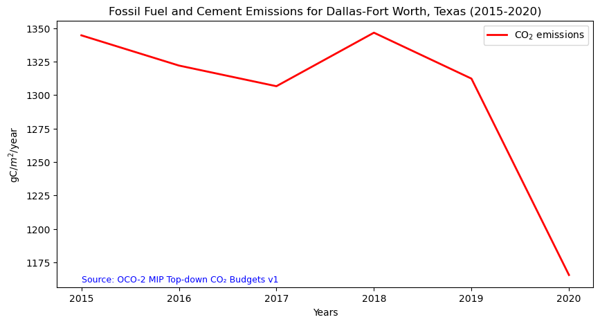
Summary
In this notebook we have successfully completed the following steps for the OCO-2 MIP Top-down CO₂ Budgets dataset:
- Install and import the necessary libraries
- Fetch the collection from STAC using the appropriate endpoints
- Count the number of existing granules within the collection
- Visualize CO₂ emissions for two distinctive years
- Generate zonal statistics for a specified region
- Plot a time series of CO₂ emission values for a specified region
If you have any questions regarding this user notebook, please contact us using the feedback form.