import numpy as np
import pandas as pd
from glob import glob
from io import StringIO
import matplotlib.pyplot as plt
import requestsAtmospheric Carbon Dioxide and Methane Concentrations from the NOAA Global Monitoring Laboratory
Atmospheric concentrations of carbon dioxide (CO₂) and methane (CH₄) from discrete air samples collected at globally distributed surface stations
Access this Notebook
You can launch this notebook in the US GHG Center JupyterHub (requires access) by clicking the following link: “Atmospheric Carbon Dioxide and Methane Concentrations from the NOAA Global Monitoring Laboratory”. If you are a new user, you should first sign up for the hub by filling out this request form and providing the required information.
If you do not have a US GHG Center Jupyterhub account, you can access this notebook through MyBinder by clicking the button below.
![]()
Table of Contents
Data Summary and Application
Atmospheric Carbon Dioxide Concentrations from the NOAA Global Monitoring Laboratory
- Spatial coverage: Global
- Spatial resolution: Point location samples
- Temporal extent: 1968 - ongoing, varies by station
- Temporal resolution: The GHG Center provides only daily and monthly means for continuous measurements; temporal resolution varies by station for non-continuous measurements (can be daily up to weekly)
- Unit: Parts CO₂ per million (ppm)
- Utility: Climate Research
Atmospheric Methane Concentrations from the NOAA Global Monitoring Laboratory
- Spatial coverage: Global
- Spatial resolution: Point location samples
- Temporal extent: 1976 - 2024, varies by station
- Temporal resolution: The GHG Center provides only daily and monthly means for continuous measurements; temporal resolution varies by station for non-continuous measurements, (can be daily up to weekly)
- Unit: Parts CH₄ per billion (ppb)
- Utility: Climate Research
For more information, visit the Atmospheric Carbon Dioxide Concentrations from the NOAA Global Monitoring Laboratory and Atmospheric Methane Concentrations from the NOAA Global Monitoring Laboratory data overview pages.
Approach
- Identify available dates and temporal frequency of observations for the given data. The collections processed in this notebook are the Atmospheric Carbon Dioxide Concentrations from the NOAA Global Monitoring Laboratory and Atmospheric Methane Concentrations from the NOAA Global Monitoring Laboratory.
- Create time-series analyses.
About the Data
Atmospheric Carbon Dioxide and Methane Concentrations from the NOAA Global Monitoring Laboratory
The Global Greenhouse Gas Reference Network (GGGRN) for the Carbon Cycle and Greenhouse Gases (CCGG) Group is part of NOAA’s Global Monitoring Laboratory (GML) in Boulder, CO. The Reference Network measures the atmospheric distribution and trends of the three main long-term drivers of climate change, carbon dioxide (CO₂), methane (CH₄), and nitrous oxide (N2O), as well as carbon monoxide (CO) and many other trace gases, which help interpretation of the main GHGs. The Reference Network measurement program includes continuous in-situ measurements at 4 baseline observatories (global background sites) and 8 tall towers, as well as flask-air samples collected by volunteers at over 50 additional regional background sites and from small aircraft conducting regular vertical profiles. The air samples are returned to GML for analysis where measurements of about 55 trace gases are done. NOAA’s GGGRN maintains the World Meteorological Organization international calibration scales for CO₂, CH₄, CO, N2O, and SF6 in air. The measurements from the GGGRN serve as a comparison with measurements made by many other international laboratories, and with regional studies. They are widely used in modeling studies that infer emission patterns and removals of greenhouse gases that are optimally consistent with the atmospheric observations, given wind patterns. These data serve as an early warning for climate “surprises”. The measurements are also helpful for the ongoing evaluation of remote sensing technologies.
For more information regarding these datasets, please visit the Atmospheric Carbon Dioxide Concentrations from the NOAA Global Monitoring Laboratory and Atmospheric Methane Concentrations from the NOAA Global Monitoring Laboratory data overview pages.
Terminology
Navigating data via the US Greenhouse Gas Center (GHGC) Application Programming Interface (API), you will encounter terminology that is different from browsing in a typical filesystem. We’ll define some terms here which are used throughout this notebook.
- collection: A specific dataset, e.g. Atmospheric Carbon Dioxide Concentrations from the NOAA Global Monitoring Laboratory
- item: One file (i.e. granule) in the dataset, e.g. a file containing daily CO₂ concentrations for a specific site
Install the Required Libraries
Required libraries are pre-installed on the US GHG Center Hub. If you need to run this notebook elsewhere, please install them with this line in a code cell:
%pip install requests folium rasterstats pystac_client pandas matplotlib –quiet
Reading the NOAA Data from GitHub Repository
First, we’ll read in the CO₂ and CH₄ concentration data from a Github repository by utilizing the Github Application Programming Interface (API). The provided endpoints refer to a location within the API that execute a request on a data collection nesting on the server.
github_repo_owner = "NASA-IMPACT"
github_repo_name = "noaa-viz"
folder_path_ch4, folder_path_co2 = "flask/ch4", "flask/co2"
combined_df_co2, combined_df_ch4 = pd.DataFrame(), pd.DataFrame()


# Function to fetch and append a file from GitHub
def append_github_file(file_url):
    response = requests.get(file_url)
    response.raise_for_status()
    return response.text

# Get the list of CH4 files in the specified directory using GitHub API
github_api_url = f"https://api.github.com/repos/{github_repo_owner}/{github_repo_name}/contents/{folder_path_ch4}"
response = requests.get(github_api_url)
response.raise_for_status()
file_list_ch4 = response.json()

# Get the list of CO2 files in the specified directory using GitHub API
github_api_url = f"https://api.github.com/repos/{github_repo_owner}/{github_repo_name}/contents/{folder_path_co2}"
response = requests.get(github_api_url)
response.raise_for_status()
file_list_co2 = response.json()
Concatenating the Data
In the next two cells, we’ll combine our CH₄ data files into one dataframe, and then do the same with the CO₂ data.
# Concatenate the CH₄ data into a single dataframe
for file_info in file_list_ch4:
    if file_info["name"].endswith("txt"):
        file_content = append_github_file(file_info["download_url"])
        Lines = file_content.splitlines()
        index = Lines.index("# VARIABLE ORDER")+2
        df = pd.read_csv(StringIO("\n".join(Lines[index:])), sep=r'\s+')
        combined_df_ch4 = pd.concat([combined_df_ch4, df], ignore_index=True)
# Concatenate the CO₂ data into a single dataframe
for file_info in file_list_co2:
if file_info["name"].endswith("txt"):
file_content = append_github_file(file_info["download_url"])
Lines = file_content.splitlines()
index = Lines.index("# VARIABLE ORDER")+2
df = pd.read_csv(StringIO("\n".join(Lines[index:])), sep=r'\s+')
combined_df_co2 = pd.concat([combined_df_co2, df], ignore_index=True)
Time-Series Analysis
Now that we have combined our data, we can plot time series analyses for the CO₂ and CH₄ concentration data. Since there are several sites that provide data, we’ll filter to only plot the data for the “ABP” or Arembepe, Bahia, Brazil site.
# Plot CO₂ concentration data
site_to_filter = 'ABP'
filtered_df = combined_df_co2[combined_df_co2['site_code'] == site_to_filter].copy()

filtered_df['datetime'] = pd.to_datetime(filtered_df['datetime'])

# Set the "Date" column as the index
filtered_df.set_index('datetime', inplace=True)

# Create a time series plot for 'Data' and 'Value'
plt.figure(figsize=(12, 6))
plt.plot(filtered_df.index, filtered_df['value'], label='Carbon Dioxide (CO₂) Concentrations (ppm)')
plt.xlabel("Observed Date/Time")
plt.ylabel("Carbon Dioxide(CO₂) Concentration (ppm)")
plt.title(f"Observed CO₂ Concentrations for the {site_to_filter} Site")
plt.legend()
plt.grid(True)
plt.show()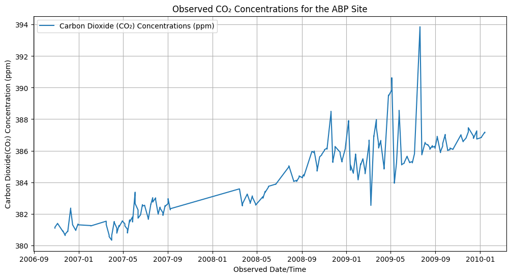
# Plot CH₄ concentration data
site_to_filter = 'ABP'
filtered_df = combined_df_ch4[combined_df_ch4['site_code'] == site_to_filter].copy()
filtered_df['datetime'] = pd.to_datetime(filtered_df['datetime'])

# Set the "Date" column as the index
filtered_df.set_index('datetime', inplace=True)

# Create a time series plot for 'Data' and 'Value'
plt.figure(figsize=(12, 6))
plt.plot(filtered_df.index, filtered_df['value'], label='Methane (CH₄) Concentrations (ppb)')
plt.xlabel("Observation Date/Time")
plt.ylabel("Methane CH₄ Concentration (ppb)")
plt.title(f"Observed CH₄ Concentrations for the {site_to_filter} Site")
plt.legend()
plt.grid(True)
plt.show()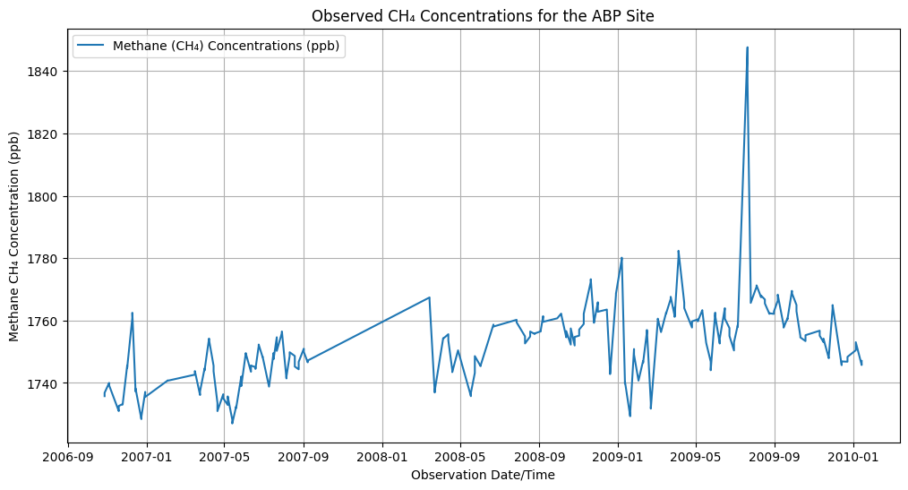
Summary
In this notebook, we have successfully completed the following steps for the Atmospheric Carbon Dioxide Concentrations from the NOAA Global Monitoring Laboratory and Atmospheric Methane Concentrations from the NOAA Global Monitoring Laboratory datasets:
- Install and import the necessary libraries
- Fetch the collections from the GitHub API using the appropriate endpoints
- Concatenate the CO₂ and CH₄ data into single dataframes
- Plot time series analyses of CO₂ and CH₄ concentration values for a specified site
If you have any questions regarding this user notebook, please contact us using the feedback form.